Full Electrical Vehicles (FEVs) and Hybrid Electrical Vehicles (HEVs) are vehicles with many electric components compared to conventional ones. In fact the power train consists of electrical machines, power electronics and electric energy storage system (battery, super capacitors) connected to mechanical components (transmissions, gear boxes and wheels) and, for HEV, to an Internal Combustion Engine (ICE). The approach for a new vehicle design has to be multidisciplinary in order to take into account the dynamic interaction among all the components of the vehicle and the power train itself. The vehicle designers in order to find the correct sizing of components, the best energy control strategy and to minimize the vehicle energy consumption need modeling and simulation since prototyping and testing are expensive and complex operations. Developing a simulation model with a sufficient level of accuracy for all the different components based on different physic domains (electric, mechanical, thermal, power electronic, electrochemical and control) is a challenge. Different commercial simulation tools have been proposed in literature and they are used by the automotive designer [1]. They have different level of detail and are based on different mathematical approaches. In paragraph 2 a general overview on different modeling approaches will be presented. In the following paragraphs the author approach, focused on the modeling of each component constituting a FEV or HEV will be detailed. The authors approach is general and is not based on vehicle oriented simulation tools. It represents a good compromise among model simplicity, flexibility, computational load and components detail representation. The chapter is organized as follows:
• paragraph 2 describes the different approaches that can be find in literature and introduced the proposed one;
• paragraphs 3 to 10 describe all the components modeling details in this order: battery, inverter, electric motor, vehicle mechanics, auxiliary load, ICE, thermal modeling;
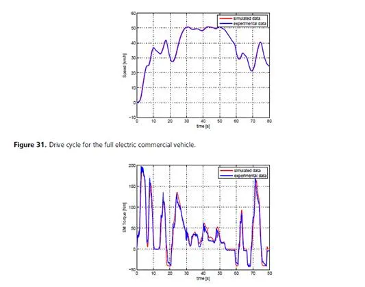
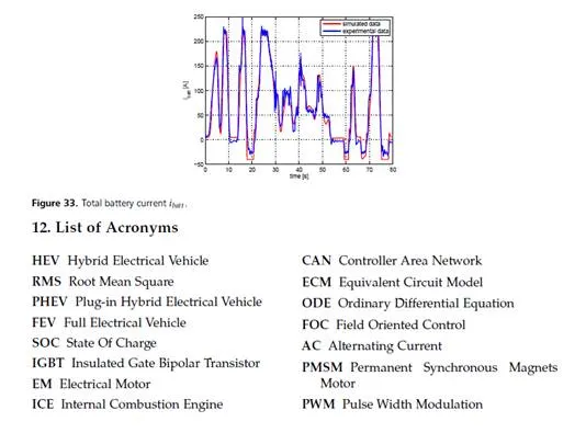
• paragraph 11 presents different cases of study with simulation results where all the numerical models has been validated by means of experimental test performed by the authors.
FEV and HEV modeling
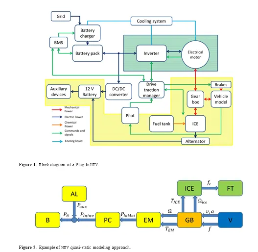
As shown in Figure 1, the whole vehicle power-train model is composed by many subsystems, connected in according to the energy and information physical exchanges. They represent the driver (pilot), the vehicle control system, the battery, the inverter, the Electrical Motor (EM), the mechanical transmission system, the auxiliary on board electrical loads, the vehicle dynamical model and for, HEVs and Plug-in Hybrid Electrical Vehicles (PHEVs), also an ICE and a fuel tank are considered. To correctly describe them, a multidisciplinary methodology analysis is required. Furthermore the design of a vehicle requires a complete system analysis including the control of the energy given from the on-board source, the optimization of the electric and electronic devices installed on the vehicle and the design of all the mechanical connection between the different power sources to reach the required performances. So, the complete simulation model has to describe the interactions between the system components, correctly representing the power flux exchanges, in order to help the designers during the study. For modeling each component, two different approaches can be used: an “equation-based” or a “map-based” mode [1]. In the first method, each subcomponent is defined by means of its quasi-static characteristic equations that have to be solved in order to obtain the output responses to the inputs. The main drawback is represented by the computational effort needed to resolve the model equations. Vice versa using a “map-based” approach each sub-model is represented by means of a set of look-up tables to numerically represents the set of working conditions. The map has to be defined by means of “off-line” calculation algorithm based on component model equation or collected experimental data. This approach implies a lighter computation load but is not parametric and requires an “off-line” map manipulation if a component parameter has to be changed. For the model developing process, an object-oriented causal approach can be adopted. In fact the complete model can be split into different subsystems. Each subsystem represents a component of the vehicle and contains the equations or the look-up table useful to describe its behavior. Consequently each object can be connected to the other objects by means of input and output variables. In this way, the equations describing each subsystem are not dependent by the external configuration, so every object is independent by the others and can be verified, modified, replaced without modify the equations of the rest of the model. At the same time, it is possible to define a “power flux” among the subsystems: every output variable of an object connected to an input signal of another creates a power flux from the first to the second subsystem (“causality approach”). This method has the advantage to realize a modular approach that allows to obtain different and complex configuration only rearranging the object connection.
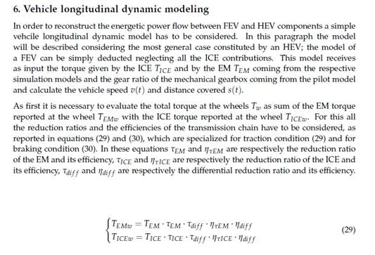
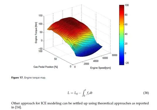
A complete model can be composed connecting the objects according two different approaches: the “reverse approach” (also called “quasi-static approach” – see Figure 2) and the “forward approach” (also called “dynamic approach” – see Figure 3). Figure 2 and 3 show simplified models of a HEV, where V is the vehicle model, GB the gear box, PC the power converter, B the battery pack, FT the fuel tank, AL is the auxiliary loads block, v and a are respectively the vehicle’s speed and acceleration, f is the vehicle traction force, Ω is the EM angular speed, TICE and TE M are respectively the ICE and the EM torques, ΩICE is the ICE angular speed, fc is the fuel consumption, I and Vs are the electrical motor current and voltage, ibatt and Vbatt are the battery current and voltage, PI n Mot is the power requested by the EM to the power converter, PB is the total power requested to the battery that is obtained as a sum of the power requested by the power converter PI n I nv and the
auxiliary loads Paux (PB = PI n I nv + Paux ) and finally iaux is the amount of current requested to the battery for auxiliary electrical loads. Quasi-static method use as input variables the desired speed and acceleration of the vehicle, hence the equations are solved starting from the V model and going back, block by block, to the B model. In the dynamic approach each subcomponent has interconnection variables with the previous and the next blocks. In this way each sub-model is strongly interleaved with the others and its behavior has influence on the total system. The second method requires a higher computational effort but is more accurate and has been applied by the authors in several cases [2–4]. In fact, using the first method, the information flux is unidirectional and the equation set is more simpler often only algebraic. This approach do not take into account the real response and constrain of power train component. On the contrary the dynamic approach produces also a response that runs
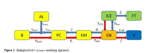
forward the complete model, influencing the output of the following sub-models. In this way, it is possible to study the total behavior including the physical limits of each component and, so, the simulation model is able to describe correctly both the single component and the overall performances of the system. For this method more complex equations (a few number of differential equation) or maps are needed. The following paragraphs describe component by component the proposed method which is based on a simplified dynamic forward approach that could be implemented using both equations or off-line computed look-up tables.
Battery modeling
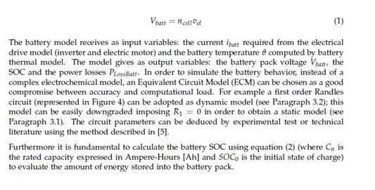
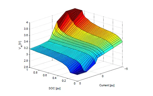
In order to correctly simulate the behavior of a FEV, HEV or PHEV it is important to set up a battery model that evaluate the output voltage considering the State Of Charge (SOC) of the battery itself. Since a battery pack is obtained by a series connection of many cells (ncell ), it is quite usual to construct a numerical model considering one single cell. The total battery voltage Vbatt is obtained using equation (1) assuming that all cells have an uniform behavior and where vel is the voltage of a single cell.
Dynamical model of battery
Since batteries for traction application are used under heavy dynamic condition with suddenly variation of the supplied current ibatt , the static model can not be adopted for all the cases of study where dynamic is fundamental (for example control analysis). Different type
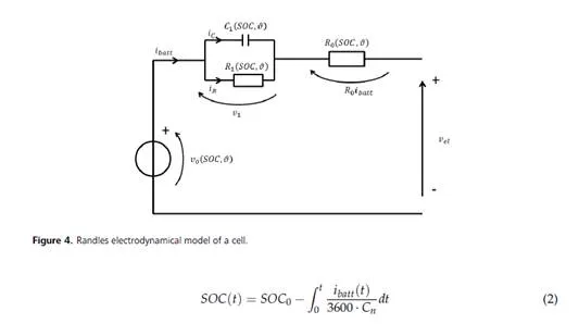
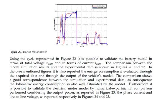
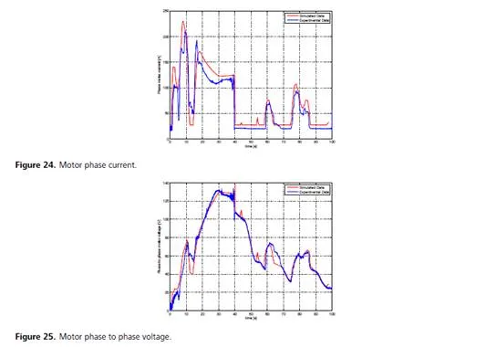
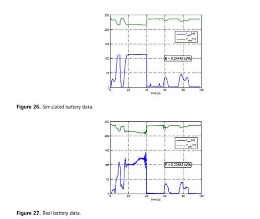
of ECM have been developed for simulating battery voltage vel where more that one RC block are used in order to obtain a Ordinary Differential Equation (ODE) of order n and a parasitic parallel branch is added to the ECM to simulate the self discharge phenomenon. Since the main objective is not to simulate all the battery details but the global vehicle behavior a single RC circuit for an enough accurate model can be adopted, as reported in Figure 4.
In order to have good simulation results a fine tuning of the dynamic ECM parameters has to be done. A good procedure for parameter identification, considering also thermal effects, is reported in [5].
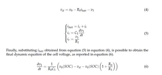
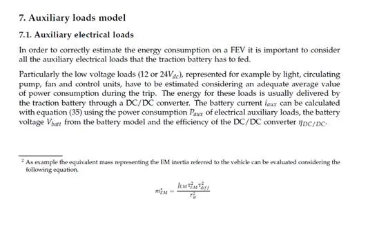
It possible to solve the circuit considering the cell voltage vel , as reported in equation (4)1 ,
![]() where the splitting of the total current ibatt into the capacitor C and into the resistor R1 is considered ad reported in equation (5) and the no load voltage v0 is SOC dependant
where the splitting of the total current ibatt into the capacitor C and into the resistor R1 is considered ad reported in equation (5) and the no load voltage v0 is SOC dependant

Comments are closed