It is well known that the injection system plays a leading role in achieving high diesel engine performance; the introduction of the common rail fuel injection system (Boehner & Kumel,
1997; Schommers et al., 2000; Stumpp & Ricco, 1996) represented a major evolutionary step that allowed the diesel engine to reach high efficiency and low emissions in a wide range of load conditions.
Many experimental works show the positive effects of splitting the injection process in several pilot, main and post injections on the reduction of noise, soot and NOx emission (Badami et al.,
2002; Brusca et al., 2002; Henelin et al., 2002; Park et al., 2004; Schmid et al., 2002). In addition, the success of engine downsizing (Beatrice et al., 2003) and homogeneous charge combustion engines (HCCI) (Canakci & Reitz, 2004; Yamane & Shimamoto, 2002) is deeply connected with the injection system performance and injection strategy.
However, the development of a high performance common rail injection system requires a considerable investment in terms of time, as well as money, due to the need of fine tuning the operation of its components and, in particular, of the electronic fuel injector. In this light, numerical simulation models represent a crucial tool for reducing the amount of experiments needed to reach the final product configuration.
Many common-rail injector models are reported in the literature. (Amoia et al., 1997; Bianchi et al., 2000; Brusca et al., 2002; Catalano et al., 2002; Ficarella et al., 1999; Payri et al., 2004). One of the older common-rail injector model was presented in (Amoia et al., 1997) and suc- cessively improved and employed for the analysis of the instability phenomena due to the control valve behaviour (Ficarella et al., 1999). An important input parameter in this model was the magnetic attraction force in the control valve dynamic model. This was calculated interpolating the experimental curve between driving current and magnetic force measured at fixed control valve positions. The discharge coefficient of the feeding and discharge control volume holes were determined and the authors asserted that the discharge hole operates, with the exception of short transients, under cavitating flow conditions at every working pressure,
but this was not confirmed by (Coppo & Dongiovanni, 2007). Furthermore, the deformation of the stressed injector mechanical components was not taken into account. In (Bianchi et al.,
2000) the electromagnetic attraction force was evaluated by means of a phenomenological model. The force was considered directly proportional to the square of the magnetic flux and the proportionality constant was experimentally determined under stationary conditions. The elastic deformation of the moving injector components were considered, but the injector body was treated as a rigid body. The models in (Brusca et al., 2002; Catalano et al., 2002) were very simple models. The aims in (Catalano et al., 2002) were to prove that pressure drops in an injection system are mainly caused by dynamic effects rather than friction losses and to analyse new common-rail injection system configurations in which the wave propagation phenomenon was used to increase the injection pressure. The model in (Brusca et al., 2002) was developed in the AMESim environment and its goal was to give the boundary conditions to a 3D-CFD code for spray simulation. Payri et al. (2004) report a model developed in the AMESim environment too, and suggest silicone moulds as an interesting tool for characteris- ing valve and nozzle hole geometry.
A common-rail injector model employs three sub-models (electrical, hydraulic and mechan- ical) to describe all the phenomena that govern injector operation. Before one can use the model to estimate the effects of little adjustments or little geometrical modifications on the system performance, it is fundamental to validate the predictions of all the sub-models in the whole range of possible working conditions.
In the following sections of this chapter every sub-model will be thoroughly presented and it will be shown how its parameters can be evaluated by means of theoretical or experimental analysis. The focus will be placed on the electronic injector, as this component is the heart of any common rail system
Mathematical model
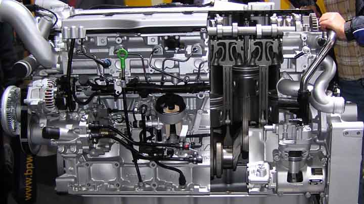
The injector considered in this investigation is a standard Bosch UNIJET unit (Fig. 1) of the common-rail type used in car engines, but the study methodology that will be discussed can be easily adapted to injectors manufactured by other companies.
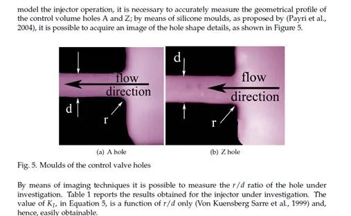
The definition of a mathematical model always begins with a thorough analysis of the parts that make up the component to be modelled. Once geometrical details and functional rela- tionships between parts are acquired and understood they can be described in terms of math- ematical relationships. For the injector, this leads to the definition of hydraulic, mechanical, and electromagnetic models.
Hydraulic Model
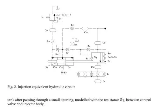
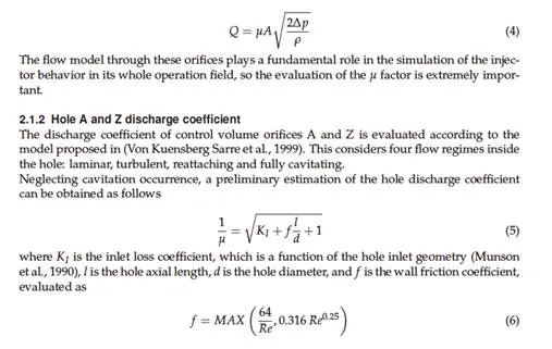
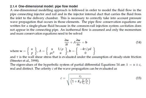
Fig. 2 shows the equivalent hydraulic circuit of the injector, drawn following ISO 1219 stan- dards. Continuous lines represent the main connecting ducts, while dashed lines represent pilot and vent connections. The hydraulic parts of the injector that have limited spatial ex- tension are modelled with ideal components such as uniform pressure chambers and laminar or turbulent hydraulic resistances, according to a zero-dimensional approach. The internal hole connecting injector inlet with the nozzle delivery chamber (as well as the pipe connect- ing the injector to the rail or the rail to the high pressure pump) are modelled according to a one-dimensional approach because wave propagation phenomena in these parts play an important role in determining injector performance.
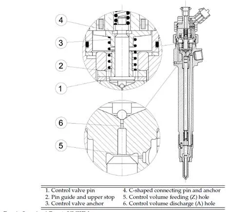
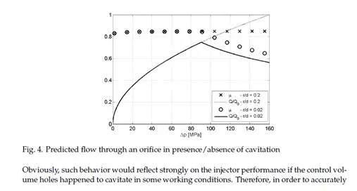
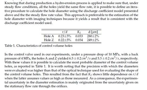
Fig. 3a shows the control valve and the relative equivalent hydraulic circuit. RA and RZ
are the hydraulic resistances used for modelling flow through control-volume orifices A (dis-
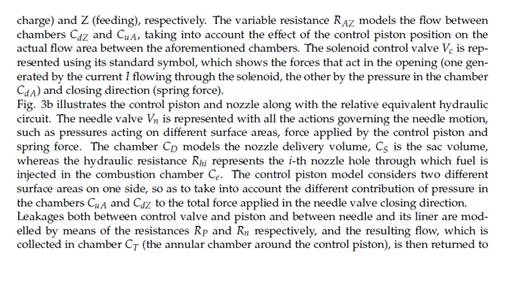
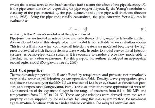
Furthermore, the leakage flow rate, Equations 2 and 3, depends on the third power of the radial gap g. At high pressure the material deformation strongly affects the gap entity and its value is not constant along the gap length l because pressure decreases in the gap when approaching the low pressure side (Ganser, 2000). In order to take into account these effects on the leakage flow rate, the value of KL has to be experimentally evaluated in the real injector working conditions.
Turbulent flow is assumed to occur in control volume feeding and discharge holes, in nozzle holes and in the needle-seat opening passage. As a result, according to Bernoulli’s law, the flow rate through these orifices is proportional to the square root of the pressure drop, ∆ p, across the orifice, namely,
Discharge coefficient of the nozzle holes
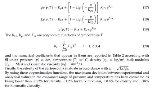
The model of the discharge coefficient of the nozzle holes is designed on the base of the un- steady coefficients reported in (Catania et al., 1994; 1997). These coefficients were experimen- tally evaluated for minisac and VCO nozzles in the real working conditions of a distributor pump-valve-pipe-injector type injection system. The pattern of this coefficient versus needle lift evidences three different phases. In the first phase, during injector opening, the moving needle tip strongly influences the efflux through the nozzle holes. In this phase, the discharge coefficient progressively increases with the needle lift. In the second phase, when the needle is at its maximum stroke, the discharge coefficient increases in time, independently from the pressure level at the injector inlet. In the last phase, during the needle closing stroke, the dis- charge coefficient remains almost constant. These three phases above mentioned describe a hysteresis-like phenomenon. In order to build a model suitable for a common rail injector in its whole operation field these three phases need to be considered.
![]()
![]() Therefore, the nozzle hole discharge coefficient is modeled as needle lift dependent by con- sidering two limit curves: a lower limit trend (µd ), which models the discharge coefficient in transient efflux conditions, and an upper limit trend (µs ), which represents the steady-state value of the discharge coefficient for a given needle lift. The evolution from transient to sta- tionary values is modeled with a first order system dynamics.
Therefore, the nozzle hole discharge coefficient is modeled as needle lift dependent by con- sidering two limit curves: a lower limit trend (µd ), which models the discharge coefficient in transient efflux conditions, and an upper limit trend (µs ), which represents the steady-state value of the discharge coefficient for a given needle lift. The evolution from transient to sta- tionary values is modeled with a first order system dynamics.
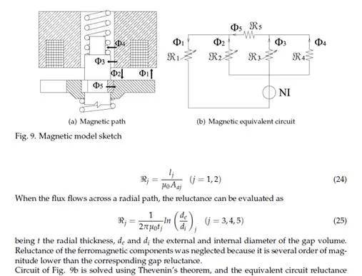
It was experimentally observed (Catania et al., 1994; 1997) that the transient trend presents a first region in which the discharge coefficient increases rapidly with needle lift, following a sinusoidal-like pattern, and a second region, characterized by a linear dependence between discharge coefficient and needle lift. Thus, the following model is adopted:
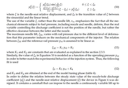
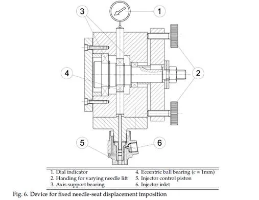
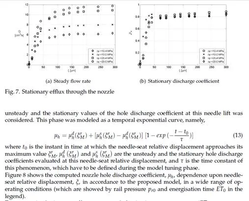
Figure 7a shows the trends of steady-state flow rate versus needle lift at rail pressures of 10 and 20 MPa, while the back pressure in the Bosch measuring tube was kept to either ambient pressure or 4 MPa; whereas Figure 7b shows the resulting stationary hole discharge coefficient, evaluated for the nozzle under investigation.
![]() Taking advantage of the reduced variation of µs with operation pressure, it is possible to
Taking advantage of the reduced variation of µs with operation pressure, it is possible to
use the measured values to extrapolate the trends of steady-state discharge coefficient for higher pressures, thus defining the upper boundary of variation of the nozzle hole discharge coefficient values.
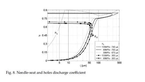
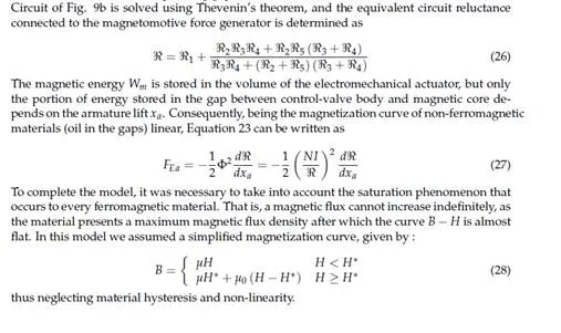
![]() During the injector opening phase the unsteady effects are predominant and the sinusoidal- linear trend of the hole discharge coefficient, Equation 10, was considered; when the needle- seat relative displacement approaches its relative maximum value ξ r , the discharge coeffi-
During the injector opening phase the unsteady effects are predominant and the sinusoidal- linear trend of the hole discharge coefficient, Equation 10, was considered; when the needle- seat relative displacement approaches its relative maximum value ξ r , the discharge coeffi-
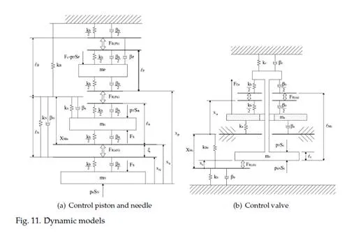
cient increases in time, which means that the efflux through the nozzle holes is moving to the stationary conditions. In order to describe this behavior, a transition phase between the
Examining the discharge coefficient, µh , trends for the three main injections (ET0 = 780 µs, 700
µs and 670 µs) during the opening phase, it is interesting to note that for a given value of the
needle lift, lower discharge coefficients are to be expected at higher operating pressures. This can be explained considering that the flow takes longer to develop if the pressure differential, and thus the steady state velocity to reach is higher.
The main injection trends also show the transition from the sinusoidal to the linear depen- dence of the transient discharge coefficient on needle lift.
The phase in which the needle has reached the maximum value and the discharge coefficient increases in time from unsteady to stationary values is not very evident in main injections, because the former increases enough during the opening phase to approach the latter. This happens because the needle reaches sufficiently high lifts as to have reduced effect on the flow in the nozzle holes, and the longer injection allows time for complete flow development. Conversely, during pilot injections (ET0 =300 µs), the needle reaches lower maximum lifts, hence lower values of the unsteady discharge coefficient, so that the phase of transition to the stationary value lasts longer. The beginning of this transition can be easily identified by analyzing the curves marked with dots and crosses in Figure 8. The point at which they depart from their main injection counterpart (same line style but without markers) marks the beginning of the exponential evolution in time to stationary value of discharge coefficient.
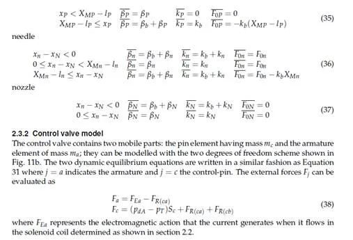
Masses, spring stiffness and damping factors
Components mass and springs stiffness k j can be easily estimated. Whenever a spring is in contact to a moving element, the moving mass mj value used in the model is the sum of the element mass and a third of the spring mass. In this way it is possible to correctly account for the effect of spring inertia too.
The evaluation of the damping factors β j in Equation 31 is considerably more difficult. Con- sidering the element moving in its liner, like needle and control piston, the damping factor takes into account the damping effects due to the oil that moves in the clearance and the fric- tion between moving element and liner. The oil flow effect can be modelled as a combined Couette-Poiseuille flow (White, 1991) and the wall shear stress on the moving element surface can be theoretically evaluated. Experimental evidences show that friction effects are more rel- evant than the fluid-dynamics effects previously mentioned. Unfortunately, these can not be theoretically evaluated because their intensity is linked to manufacturing tolerances (both ge- ometrical and dimensional). Therefore, damping factors must be estimated during the model tuning phase.
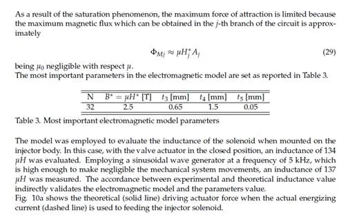
Model tuning and results
Any mathematical model requires to be validated by comparing its results with the experi- mental ones. During the validation phase some model parameters, which cannot be experi- mentally or theoretically evaluated, have to be carefully adjusted.
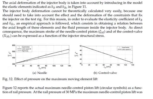
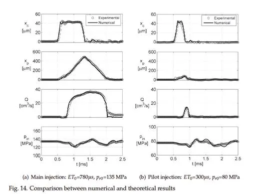
The model here presented was tested comparing numerical and experimental control valve lift xc , control piston lift xP , injected flow rate Q and injector inlet pressure pin in several operating conditions. Figure 15 shows two of these validation tests and the good accordance between experimental and numerical results is evident.
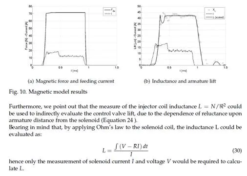
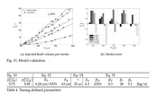
Table 4 shows the value of the parameters that were adjusted during the tuning phase. These values can be used as starting points for the development of new injector models, but their exact value will have to be defined during model tuning for the reasons explained above. After the tuning phase the model can be used to reproduce the injection system performance in its whole operation field. By way of example, Fig. 15 shows the experimental and numerical volume injected per stroke Vf and the percentage error of the numerical estimation.

Comments are closed