IPG CarMaker is a simulation environment used to simulate a computer representation of a real vehicle with the behaviour matching the real vehicle. In this environment, the user creates the vehicle using mathematical models that contain equations of motion kinematics, but also a multi‐body definition of the system. The parameters are modified in accordance with the real vehicle to be studied [1].

IPG CarMaker is also used for other purposes than just pure simulation, which are as follows: it is coupled with MATLAB in order to implement new algorithms, for example vehicle state estimation using an integrated Kalman filter scheme for vehicle dynamics estimation (side slip) [2]; it is used as model‐predicting control for fuel consumption optimization of a range extender for a hybrid vehicle architecture (state of charge trajectory estimation) [3]; it is used as a validation of a controller for variable steering ratio of a front steering system, tested on a virtual road for driving comfort improvement [4]; it is used for solving challenging problems such as wheel slip control for electric powertrain vehicles, for anti‐lock brake and traction control functional validation (hardware‐in‐the‐loop (HIL) using IPG CarMaker coupled with dSPACE) [5] and complex hardware‐in‐the‐loop system (MATLAB Simulink model coupled with IPG CarMaker multibody vehicle model, dSPACE electronic control unit, and a real friction brake unit) for brake friction optimization and lower energy consumption [6].

Using this knowledge, it is possible to simulate any vehicle in IPG CarMaker, as long as the user knows all the necessary data. The same behaviour can be simulated for any vehicle, on the same road, with the same manoeuvres, just by changing the vehicle properties. The vehicle contains all components from the real vehicle, such as powertrain, chassis, tires, brakes, but also controllers, such as ABS (Anti-Lock Braking System), ESP (Electronic Stability Program), ACC (Adaptive Cruise Control), or other user‐modelled systems.

After defining the virtual vehicle, the user must characterize the road, that is a digitized or computer‐modelled representation of the real road (usual road, track, or course), which simulates the road and it is generated for testing. CarMaker can generate the road using the following two methods:

·         An easy method that combines individual road segments, such as straights and curves, to form a continuous road, where all the parameters interconnect. For each segment, the user can define all the data such as angle, slope, pitch, friction coefficient, length, and width.

·         The second method involves an existing road file (already digitized data), generated by a direct measurement from a GPS device, Google Earth, or other. The file can be opened by CarMaker and used as the road or track during simulation.

The third step is defining the virtual driver, which simulates the actions of a real driver. All the parameters would normally be controlled by a real driver, such as turning/steering or operating the gas, brake and clutch pedals, shifting gears (for manual transmission). For the virtual driver, there are two approaches in CarMaker:

·         A simply controlled driver, for which the user can specify at each step what the virtual driver should do.

·         An IPG driver, a smart‐controlled driver, which tries to maintain the given trajectory and operate within specified limits. As an example, the reaction time can be modified.

Altogether, the virtual vehicle, the virtual driver, and the virtual road form the virtual vehicle environment.

CarMaker also has the CIT (CarMaker interface toolbox) that consists of a number of tools that run on a host computer, namely:

·         IPG control—it is a visualization and analysis tool that can monitor quantities in real‐time, load post‐simulation data, plot, and export results;

·         CarMaker GUI—it is a main graphical user interface that controls the virtual vehicle environment, where the user can select all the virtual parameters (virtual vehicle, virtual road, virtual driver parameters, load manoeuvres);

·         Vehicle data set editor—it allows the user to control and modify all the parameters of the vehicle;

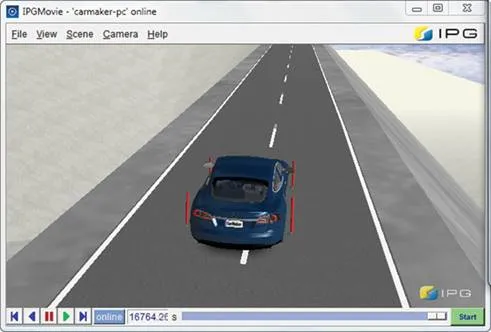
·         IPGMovie—it shows a real‐time 3D animation of the vehicle performing the desired manoeuvres on the specified road;

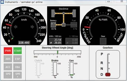
·         Instrumentsit shows the important instruments like dials, and information about driving conditions such as position on the pedals, ABS warning lamp, brake light and others;

·         Direct variable access (DVA)—allows the simulation quantities to be viewed and modified interactively;

·         ScriptControl—it is a test automation utility that allows scripts to be defined, edited, and executed. All the functions of the CIT can be controlled automatically using ScriptControl;

·         TestManager—it is another utility for test automation. A mixture of script and GUI‐based creation and execution of test series.

The vehicle that was chosen for the simulation is a Tesla Model S because it is an electric car with a good range (currently using an 85‐kWh battery, from which a range of 426 km can be achieved and an energy consumption of 237.5 Wh/km) [7].

Creating a simulation

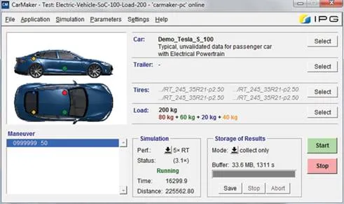
Creating a simulation involves using the CIT to create the desired model of the real situation that needs to be simulated, choosing the vehicle (with all its properties), the driver, the road, the manoeuvres and the load (Figure 1).

Before actually starting the simulation, the Instruments window should be activated (Figure 2), the IPGMovie window to visualize the status in real time (or faster) and more importantly (Figure 3), and the IPG Control Data window to observe the evolution of certain parameters and save results.

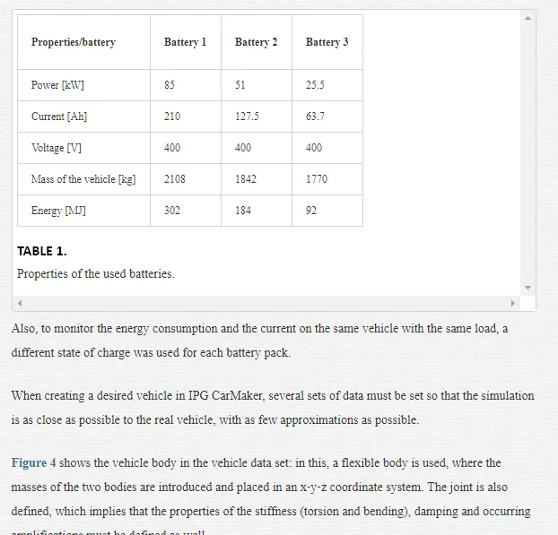
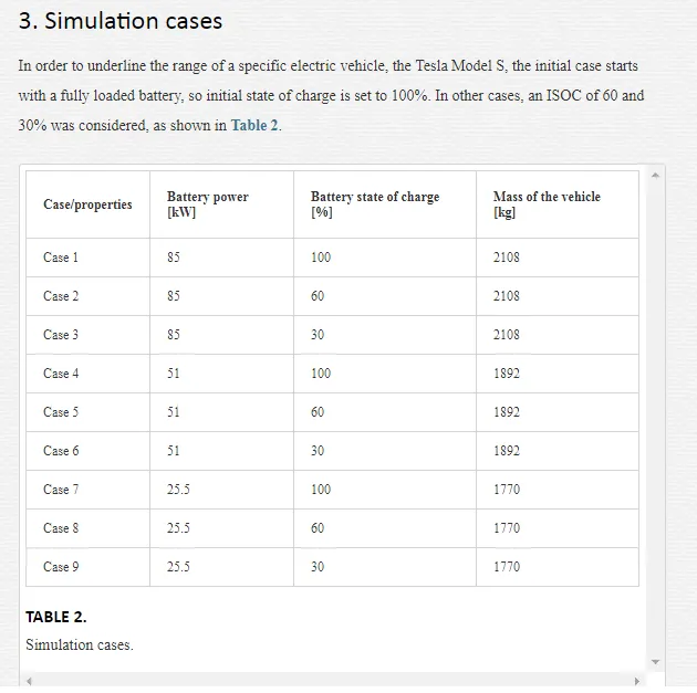
Also, to monitor the energy consumption and the current on the same vehicle with the same load, a different state of charge was used for each battery pack.

When creating a desired vehicle in IPG CarMaker, several sets of data must be set so that the simulation is as close as possible to the real vehicle, with as few approximations as possible.

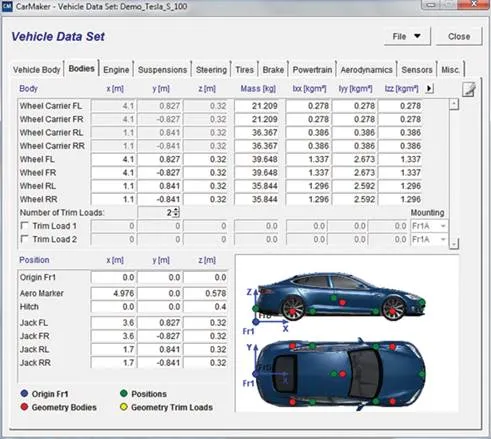
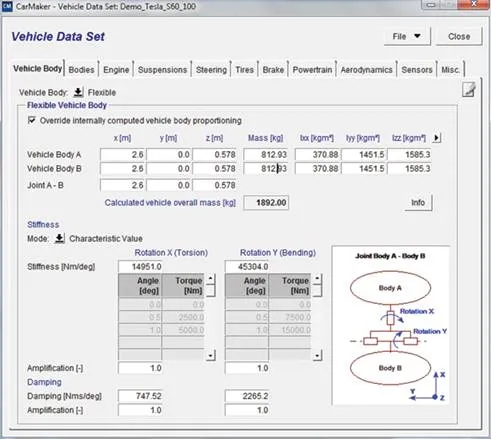
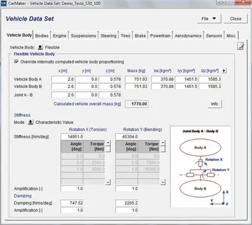
Figure 4 shows the vehicle body in the vehicle data set: in this, a flexible body is used, where the masses of the two bodies are introduced and placed in an x‐y‐z coordinate system. The joint is also defined, which implies that the properties of the stiffness (torsion and bending), damping and occurring amplifications must be defined as well.

After the properties of the vehicle body are done, the next required input is the vehicle bodies (Figure 5), where the required fields are moments of inertia for all wheel carriers, for all the wheels, placements of the wheels, hitch position if required and, if any, trim loads. In this case, there are no trim loads.

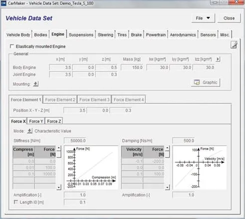
Since it is an electric car, no internal combustion engine was input (Figure 6). This feature can be used if the simulation requires a hybrid vehicle or a classic vehicle.

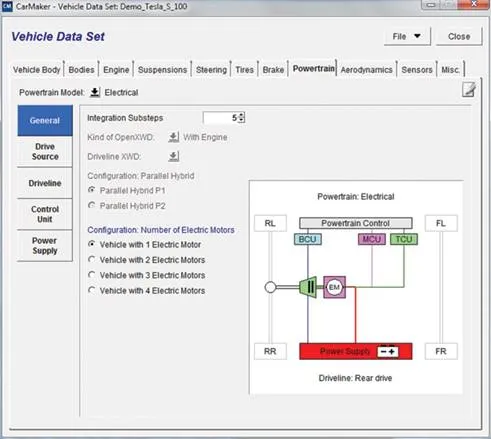
When simulating an electric vehicle, after introducing the required data for suspension, steering, tires, and brakes, the powertrain data are extremely important: in the general submenu, the number of electric motors is selected—in this case, one electric motor (Figure 7).

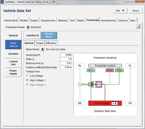
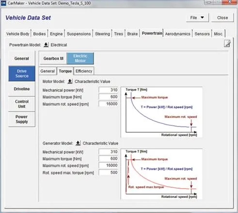
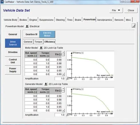
In the second submenu, drive source, the general data are introduced such as moment of inertia for the electric motor, ratio, build‐up time, friction coefficient, and voltage level (Figure 8), but also the torque (as a characteristic value) for both cases of the electric motor (motor or generator), as shown in Figure 9, and the efficiencies of the electric motor in both cases (Figure 10).

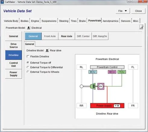
The next input is the driveline: the rear drive option was selected by this, with no external torque (Figure 11), because it is not the case since there is no external torque to the differential or wheels.

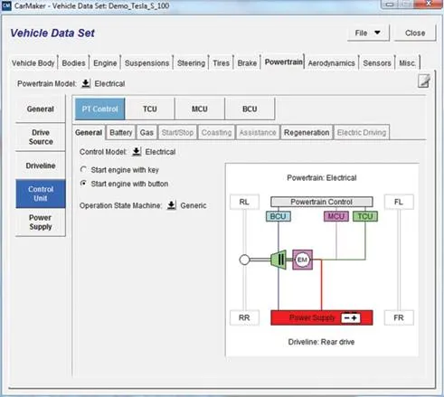
For the control unit, first the powertrain control is set to electrical, the engine start with button and not key, and the desired input for the body control unit (BCU), motor control unit (MCU), and traction control unit (TCU), as shown in Figure 12.

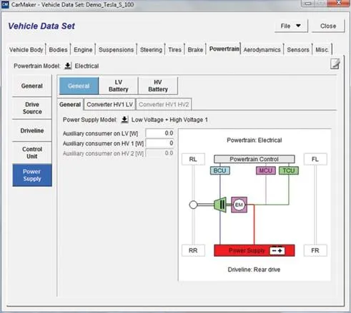
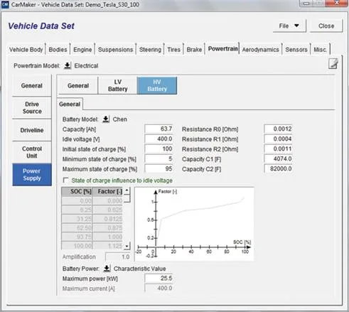
For the electric vehicle, the power supply is of most importance: low voltage, high voltage or both low voltage and high voltage can be selected; in this case, low and high voltages were selected with no auxiliary consumer for neither low nor high voltage (Figure 13).

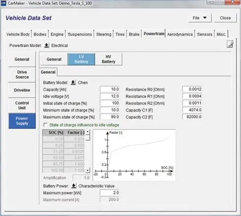
In the low voltage set‐up menu, the main data regarding the LV battery can be introduced, such as capacity, idle voltage, initial state of charge (ISOC), minimum and maximum state of charge, capacities and resistances of the battery (Figure 14).

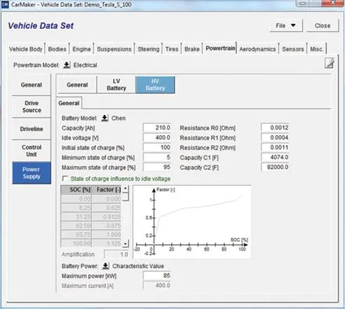
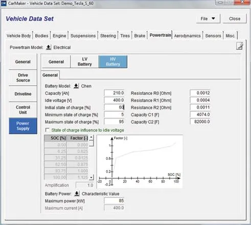
For the high‐voltage battery, the current state (as on the real vehicle) is inserted, a battery with the capacity of 210 Ah, 85 kW of power, idle voltage of 400 V, and the specific resistances and capacities of the battery (Figure 15

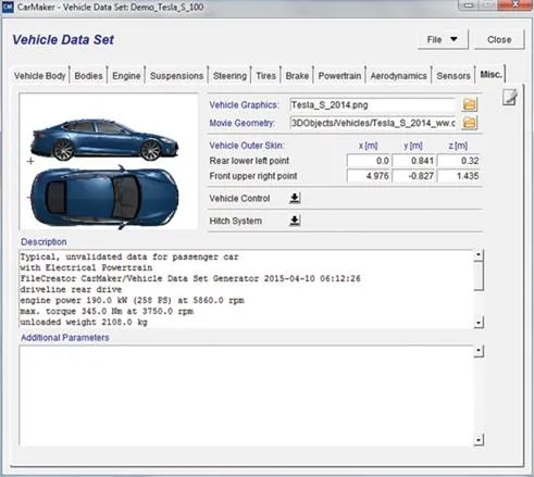
In the miscellaneous menu, the vehicle graphics and the movie geometry (in order to create a proper video in real time of the desired vehicle: Tesla Model S) were selected (Figure 16).

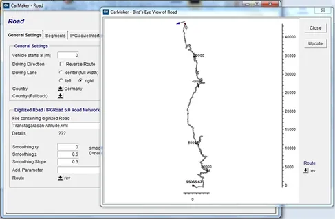
After the vehicle is ready, the input for the road follows (Figure 17) where the driver must maintain a constant speed and the manoeuvres are just to follow the given road.

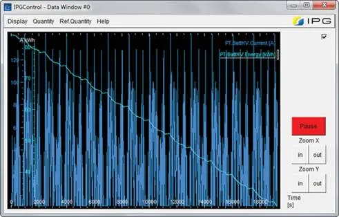
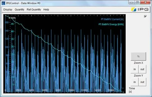
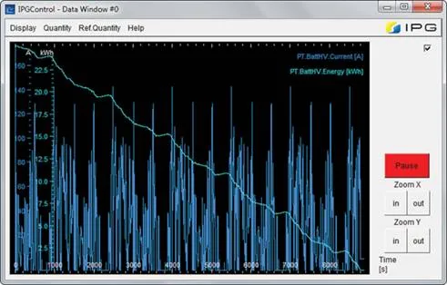
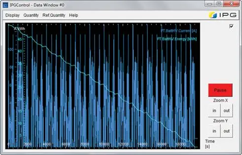
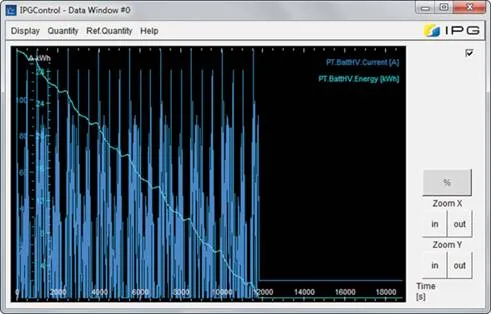
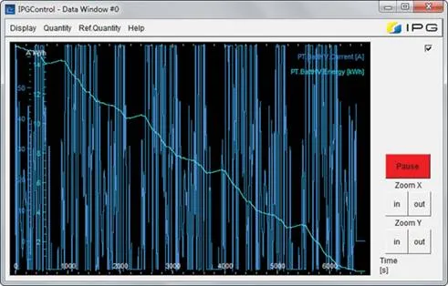
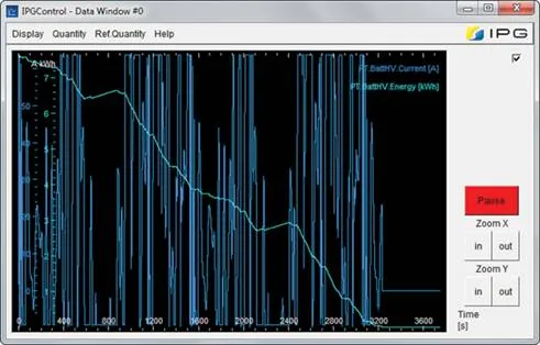
After creating the Case 1 Model, the simulation is started, and the results of the battery current and energy can be monitored in the DataWindow (Figure 18). After the vehicle stops, the distance is recorded and the state of charge of the battery is changed (Figure 19), with new results (Figure 20) and the same is done for case 3 (Figure 21).

In order to change the data for Cases 4–6, the mass of the vehicle bodies was modified so that the total mass of the vehicle is correct for these cases (1892 kg) as shown in Figure 22, but also the maximum power was reduced to 51 kW (Figure 23), with results shown in Figure 24 (Case 4), Figure 25 (Case 5), and Figure 26 (Case 6).

For Cases 7–9, the mass of the vehicle bodies was modified so that the total mass of the vehicle is correct (1770 kg) as shown in Figure 27, but also the maximum power was reduced to 25.5 kW (Figure 28), with results shown in Figure 29 (Case 7), Figure 30 (Case 8), and Figure 31 (Case 9)

Results

After each simulation, the range was recorded, and the battery current and energy were monitored via DataWindow. All data from the DataWindow can be exported as separate files and evaluated.

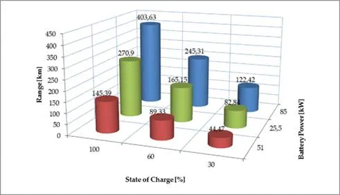
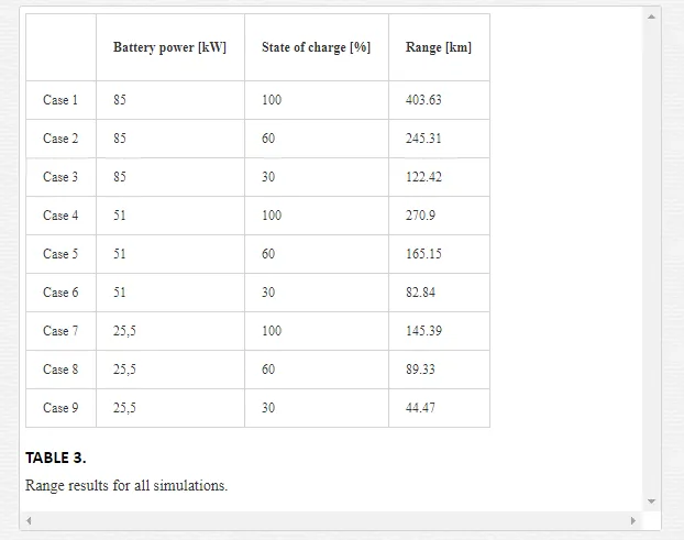
The results regarding the range are presented in Table 3, and as a graph in Figure 31.

In order to see how these results were obtained, the energy consumption has to be monitored:

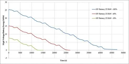
·         Energy consumption for all SOC with the 25.5‐kW battery (Figure 32);

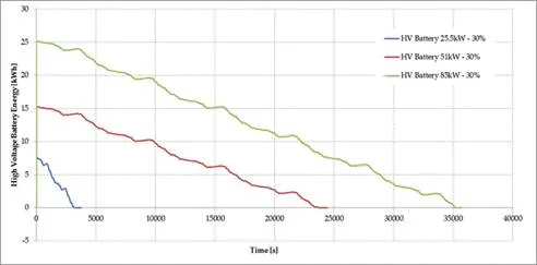
·         Energy consumption for 30% SOC with all batteries (Figure 33).

Conclusion

IPG CarMaker is a powerful simulation tool that can estimate, due to its complexity and number of input factors, output values very close to reality; just as in Case 1, where the maximum range of the Tesla Model S is 403.63 km, close to the specifications of the producer [7].

It can be seen in the simulations that the range of the vehicle increases with the state of charge of the battery; when the power of the battery is decreased, the range decreases because of the lower power, but also increases due to the lower weight of the vehicle; overall, the range decreases.

When analysing Figure 33, the energy of the batteries has similar slopes for the 85 and 51 kW batteries, but the slope for the smallest battery, 25.5 kW is more abrupt, decreasing fast in comparison to the others.

The answer to the initial question—what is the correct number of batteries that a vehicle must equip in order to have a bigger range—is as many as possible, limited by the final price of the vehicle, even though the tendencies in the batteries domain are to reduce the weight as much as possible and store as much energy as possible.

IPG CarMaker is a SIL (simulation in the loop) software that takes into account all reactions from the road and from the transmission and adapts the driver behaviour.

By connecting it to a real engine testbed or powertrain testbed, the IPG CarMaker can be transformed into a HIL (hardware‐in‐the‐loop) simulation, where the behaviour of the real engine is controlled by the virtual driver, on the virtual road, from the virtual vehicle and the response of the load is controlled by adjusting the dynamometer load.