Fuel Consumption and CO2 Emissions
These days the detrimental effects of air pollutants and concerns about global warming are being increasingly reported by the media. In many countries, fuel prices have been rising considerably. In western Canada, for instance, the gasoline price almost doubled from about 53 cents/liter in 1998 to 109 cents/liter in 2010 (Wiebe, 2011). In terms of the air pollution problem, greenhouse gas (GHG) emissions from vehicles are considered to be one of the main contributing sources. Carbon dioxide (CO2 ) is the largest component of GHG emissions. For example, in Japan in 2008, the amount of CO2 emissions from vehicles (200 million ton) is about 17 percent of the entire CO2 emissions from Japan (1200 million ton) (Tsugawa & Kato, 2010). The Kyoto Protocol aims to stabilize the GHG concentrations in the atmosphere at a level that would prevent dangerous alterations to the regional and global climates (OECD/IEA, 2009). As a result, it is important to develop and implement effective strategies to reduce fuel expenditure and prevent further increases in CO2 emissions from vehicles.
A significant amount of fuel consumption and emissions can be attributed to drivers getting lost or not taking a very direct route to their destination, high acceleration, stop-and-go conditions, congestion, high speeds, and outdated vehicles. Some of these cases can be alleviated by implementing Intelligent Transportation Systems (ITS).
ITS is an integration of software, hardware, traffic engineering concepts, and communication technology that can be applied to transportation systems to improve their efficiency and safety (Chowdhury & Sadek, 2003). In ITS technology, navigation is a fundamental system that helps drivers select the most suitable path. In (Barth et al., 2007), a navigation tool has been designed especially for minimizing fuel consumption and vehicle emissions. A number of scheduling methods have been proposed to alleviate congestion (Kuriyama et al., 2007) as vehicles passing on an uncongested route often consume less fuel than the ones on a congested route (Barth et al., 2007).
Various forms of wireless communications technologies have been proposed for ITS. Vehicular networks are a promising research area in ITS applications (Moustafa & Zhang, 2009), as drivers can be informed about many kinds of events and conditions that can impact travel.

To exchange and distribute messages, broadcast and geocast routing protocols have been proposed for ITS applications (Broustis & Faloutsos, 2008; Sichitiu & Kihl, 2008) to evaluate network performance (e.g., message delays and packet delivery ratio), instead of evaluating the impact of the protocols on the vehicular system (e.g., fuel consumption, emissions, and travel time).
This chapter studies the impact of using a geocast protocol in vehicular networks on the vehicle fuel consumption and CO2 emissions. Designing new communication protocols that are suitable in applications, such as reducing vehicle fuel consumption and emissions, is out of this chapter ’s scope. The purpose of this chapter is to:
• Motivate researchers working in the field of communication to design economical and environmentally friendly geocast (EEFG) protocols that focus on minimizing vehicle fuel consumption and emissions;
• Demonstrate the ability to integrate fuel consumption and emission models with vehicular networks;
• Illustrate how vehicular networks can be used to reduce fuel consumption and CO2
emission in a highway and a city environment.
This research brings together three key areas which will be covered in Sections 2, 3, and 4. These areas are: (1) geocast protocols in vehicular networks; (2) vehicle fuel consumption and emission models; and (3) traffic flow models. Section 5 will introduce two scenarios where applying vehicular networks can reduce significant amounts of vehicle fuel consumption and CO2 emissions.
Geocast protocols in vehicular networks
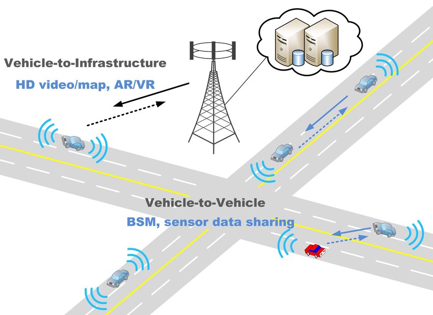
Geocast protocols provide the capability to transmit a packet to all nodes within a geographic region. The geocast region is defined based on the applications. For instance, a message to alert drivers about congestion on a highway may be useful to vehicles approaching an upcoming exit prior to the obstruction, yet unnecessary to vehicles already in the congested area. As shown in Figure 1, the network architectures for geocast in vehicular networks can be Inter-Vehicle Communication (IVC), infrastructure-based vehicle communication, and Hybrid Vehicle Communication (HVC). IVC is a direct radio communication between vehicles without control centers. Thus, vehicles need to be equipped with network devices that are based on a radio technology, which is able to organize the access to channels in a decentralized manner (e.g., IEEE 802.11 and IEEE 802.11p). In addition, multi-hop routing protocols are required, in order to forward the message to the destination that is out of the sender ’s transmission range. In infrastructure-based vehicle communication, fixed gateways are used for communication such as access points in a Wireless Local Area Network (WLAN). This network architecture could provide different application types and large coverage. However, the infrastructure cost has to be taken into account. HVC is an integration of IVC with infrastructure-based communications.
The existing geocast protocols are classified based on the forwarding types, which are either simple flooding, efficient flooding, or forwarding without flooding (Maihöfer, 2004). In this chapter, geocast protocols are classified based on performance metrics. An important goal of vehicular networks is to disseminate messages with low latency and high reliability. Therefore, most existing geocast protocols for vehicular networks aim to minimize message
Geocast protocols aim to minimize message latency
Message latency can be defined as the delay of message delivery. A higher number of wireless hops causes an increase in message latency. Greedy forwarding can be used to reduce the number of hops used to transmit a packet from a sender to a destination. In this approach, a packet is forwarded by a node to a neighbor located closer to the destination (Karp & Kung,
2000). Contention period strategy can potentially minimize message latency. In reference (Briesemeister et al, 2000), when a node receives a packet, it waits for a period of time before rebroadcast. This waiting time depends on the distance between the node and the sender; as such, the waiting time is shorter for a more distant receiver. The node will rebroadcast the packet if the waiting time expires and the node did not receive the same packet from another node. Otherwise, the packet will be discarded.
Geocast protocols aim to increase the dissemination reliability
One of the main problems associated with geocast routing protocols is that these protocols do not guarantee reliability, which means not all nodes inside a geographic area can be reached. Simple flooding forwarding can achieve a high delivery success ratio because it has high transmission redundancy since a node broadcasts a received packet to all neighbors. However, the delivery ratio will be worse with increased network size. Also, frequent broadcast in simple flooding causes message overhead and collisions. To limit the inefficiency of the simple flooding approach, directed flooding approaches have been proposed by
1. Defining a forwarding zone;
2. Applying a controlled packet retransmission scheme within the dissemination area.
Location Based Multicast (LBM) protocols are based on flooding by defining a forwarding zone. In reference (Ko & Vaidya, 2000), two LBM protocols have been proposed. The first protocol defines the forwarding zone as the smallest rectangular shape that includes the sender and destination region. The second one is a distance-based forwarding zone. It defines the forwarding zone by the coordinates of sender, destination region, and distance of a node to the center of the destination region. An intermediate node broadcasts a received packet only if it is inside the forwarding zone. Emergency Message Dissemination for Vehicular environment (EMDV) protocol requires the forwarding zone to be shorter

than the communication range and to lie in the direction of dissemination (Moreno, 2007). The forwarding range is adjusted according to the probability of reception of a single hop broadcast message. In this case, high reception probability near the boundary of the range can be achieved.
A retransmission counter (RC) is proposed as a packet retransmission scheme (Moreno, 2007). When nodes receive a packet, they cache it, increment the RC and start a timer. RC=0 means the node did not receive the packet correctly. The packet will be rebroadcast if the time is expired. Moreover, the packet will be discarded if the RC reaches a threshold.
For small networks, temporary caching can potentially increase the reliability (Maihofer & Eberhardt, 2004). The caching of geounicast packets is used to prevent the loss of packets in case of forwarding failures. Another type of caching is for geobroadcast which is used to keep information inside a geographical area alive for a certain of time.
Geocast protocols aim to reduce vehicle fuel consumption and emissions
To the best of our knowledge, all existing protocols focus on improving the network-centric performance measures (e.g., message delay, packet delivery ratio, etc.) instead of focusing on improving the performance metrics that are meaningful to both the scientific community and the general public (e.g., fuel consumption, emissions, etc.). The key performance metrics of this chapter are vehicle fuel consumption and CO2 emissions. These metrics can be called economical and environmentally friendly (EEF) metrics.
Improving the network metrics will improve the EEF metrics. However, the existing protocols are not EEF because their delivery approach and provided information are not designed to assist vehicles in reducing uneconomical and environmentally unfriendly (UEF) actions. These actions include
• Acceleration;
• High speed;
• Congestion;
• Drivers getting lost or not taking a very direct route to their destination;
• Stop-and-go conditions;
• Idling cars on the road;
• Choosing a path according to a navigation system that later becomes congested and inefficient after committing to that path.
Fuel consumption and emission models
A number of research efforts have attempted to develop vehicle fuel consumption and emission models. Due to their simplicity, macroscopic fuel consumption and emission models have been proposed (CARB, 2007; EPA, 2002). Those models compute fuel consumption and emissions based on average link speeds. Therefore, they do not consider transient changes in a vehicle’s speed and acceleration levels. To overcome this limitation, microscopic fuel consumption and emission models have been proposed (Ahn & Rakha, 2007; Barth et al.,
2000), where a vehicle fuel consumption and emissions can be predicted second-by-second. An evaluation study has been applied on a macroscopic model called MOBILE6 and two microscopic models: the Comprehensive Modal Emissions Model (CMEM) and the Virginia
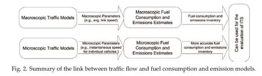
Tech Microscopic model (VT-Micro) (Ahn & Rakha, 2007). It has been demonstrated that
the VT-Micro and CMEM models produce more reliable fuel consumption and emissions
estimates than the MOBILE6 (EPA, 2002). Figure 2 shows the link between transportation
models and fuel consumption and emissions estimates.
Microscopic models are well suited for ITS applications since these models are concerned with
computing fuel consumption and emission by tracking individual vehicles instantaneously.
The following subsections briefly describe the two widely used microscopic models.
CMEM model
The development of the CMEM began in 1996 by researchers at the University of California,
Riverside. The term “comprehensive” is utilized to reflect the ability of the model to
predict fuel consumption and emissions for a wide variety of vehicles under various
conditions. The CMEM model was developed as a power-demand model. It estimates about
30 vehicle/technology categories from the smallest Light-Duty Vehicles (LDVs) to class 8
Heavy-Duty Trucks (HDTs) (Barth et al., 2000). The required inputs for CMEM include vehicle
operational variables (e.g., second-by-second speed and acceleration) and model-calibrated
parameters (e.g., cold-start coefficients and engine-out emission indices). The cold-start
coefficients measure the emissions that are produced when vehicles start operation, while
engine-out emission indices are the amount of engine-out emissions in grams per one gram
of fuel consumed (Barth et al., 2000; UK, 2008). The CMEM model was developed using
vehicle fuel consumption and emission testing data collected from over 300 vehicles on three
driving cycles, following the Federal Test Procedure (FTP), US06, and the Model Emission
Cycle (MEC). Both second-by-second engine-out and tailpipe emissions were measured.
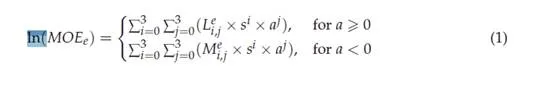
VT-Micro model
The VT-Micro model was developed using vehicle fuel consumption and emission testing data
obtained from an experiment study by the Oak Ridge National Laboratory (ORNL) and the
Environmental Protection Agency (EPA). These data include fuel consumption and emission
rate measurements as a function of the vehicle’s instantaneous speed and acceleration
levels. Therefore, the input variables of this model are the vehicle’s instantaneous speed
and acceleration. The model was developed as a regression model from experimentation
with numerous polynomial combinations of speed and acceleration levels as shown in the
following equation.
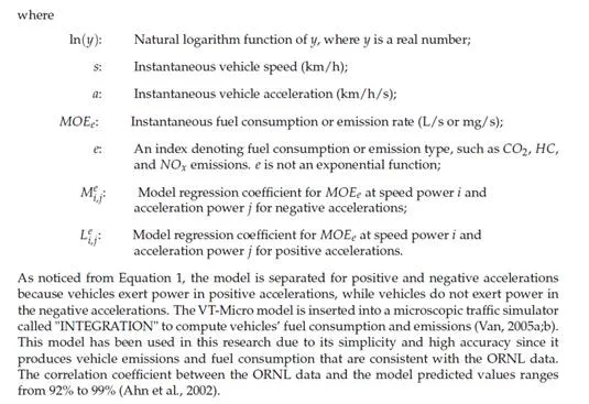
Example of using the VT-Micro model
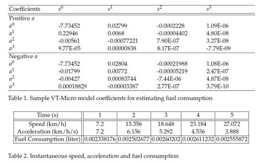
Sample model coefficients for estimating fuel consumption rates for a composite vehicle are introduced in Table 1. The composite vehicle was derived as an average across eight light-duty vehicles. The required input parameters of the model are:
• Instantaneous speed (km/h);
• Instantaneous acceleration (km/h/s);
• Model regression coefficient for positive and negative acceleration as given in Table 1.
Consider a vehicle started traveling. A microscopic traffic model has to be utilized in order to measure the vehicle instantaneous speed and acceleration. Simulation of Urban Mobility (SUMO) has been used in this regard. SUMO is a microscopic traffic simulation package developed by employees of the Institute of Transportation Systems at the German Aerospace Center (Krajzewicz et al., 2002).
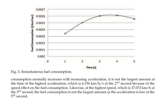
VT-Micro model has a speed-acceleration boundary. For instance, at speed 50 km/h, the maximum acceleration that can be used in the model is around 2.2 m/s2 (Ahn et al., 2002). In this example, the maximum vehicle speed, acceleration and deceleration are set to 50 km/h, 2 m/s2 and -1.5 m/s2 , respectively. The second-by-second speed and acceleration are computed for the first 5 seconds of the vehicle’s trip as shown in Table 2. It is noticed that all accelerations are positive. By applying the input parameters to Equation 1, the fuel consumption estimates should be as demonstrated in Table 2 and Figure 3. Clearly from the table, the increase or decrease of the fuel consumption is based on the speed and acceleration. Although fuel
Example of a cellular automata model of car traffic
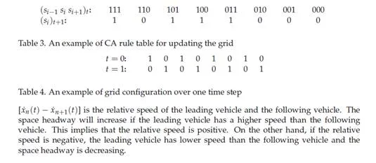
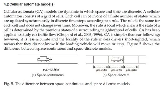
The model in this example is for a one-way street with one lane. The street is divided into cells. Each cell can be in one of two states (s). The first state represents an empty cell, denoted “0″, while the second state represents a cell occupied by a vehicle, denoted “1″. The movements of the vehicles are simulated as they jump from one cell to another (i → i + 1). The rule is that a vehicle jumps only if the next cell is empty. Consequently, the state of a cell is determined based on the states of its neighbors. In this model, each cell has two neighbors: one to its direct right, and one to its direct left. The car motion rule and the grid configuration over one time step can be explained as in Table 3 and Table 4, respectively.
The fraction of cars able to move is the number of motions divided by the total number of cars. For instance, in Table 4 at t=0, the number of motions is similar to the total number of
Geocast in vehicular networks for optimum reduction of vehicles’ fuel consumption and emissions
By means of two examples, we show how vehicular networks can be used to reduce fuel consumption and carbon dioxide (CO2 ) emission in a highway and a city environment. The first example is in a highway environment with the fuel consumption as the performance metric (Alsabaan et al., 2010a). The second example is in a city environment with considering the CO2 emission as the performance metric (Alsabaan et al., 2010b).
Highway environment
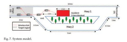
Considering two highways (Hwys) and an accident occurred, this example illustrates the necessity of transmitting information to vehicles in order for drivers to choose the economical path. Simulation results demonstrate that significant amounts of fuel will be saved if such an economical geocast (EG) protocol is used.
System model
Since this work is quite interdisciplinary, models from different areas have to be considered. The system model includes (1) traffic model: represents the characteristics of the road network; (2) accident model: represents the characteristics of the accident; (3) fuel consumption and emission model: estimates the amount of fuel consumption and CO2 emissions from vehicles; (4) communication model: represents the communication components and technologies that can be used for such an application.
Fuel Consumption and Emission Model: The VT-Micro model has been used in this example due to its simplicity and high accuracy. This model produces vehicle fuel consumption and emissions that are consistent with the ORNL data. The correlation coefficient between the ORNL data and the model predicted values ranges from 92% to
99% (Ahn et al., 2002). A more detailed description of the model is provided in Subsection
3.2.
Communication Model: Assume the existence of Inter-Vehicle Communication (IVC). Each vehicle is equipped with an Application Unit (AU) and On-Board Unit (OBU). It is assumed in this study that the AU can detect the crash occurrence of its vehicle. Moreover, it is assumed that the AU is equipped with a navigation system. It is also assumed in this example that the OBU is equipped with a (short range) wireless communication device. A multi-hop routing protocol is assumed in order to allow forwarding of data to the destination that has no direct connectivity with the source.
In this example, the use of geographical positions for addressing and routing of data packet (geocast) is assumed. The destination is addressed as all nodes in a geographical region. Designing or proposing the communication protocols that are suitable in applications such as reducing fuel consumption is out of the scope of this example. The main objective of this example is to encourage communications researchers to propose protocols with a goal of minimizing vehicle fuel consumption.
Simulation study
The lengths of the highways and accident are shown in Figure 7. Hwy 1 and Hwy 2 are 4-lane one direction. For both highways, the free-flow speed is 90 km/h. One of the important road segment characteristics is its basic saturation flow rate which is the maximum number of vehicles that would have passed the segment after one hour per lane. Another important characteristic is the speed at the basic saturation flow or speed-at-capacity. In this study, the basic saturation flow rate per lane is 2000 vehicles per hour with speed 70 km/h.
Vehicles enter the system uniformly in terms of the vehicle headway with a rate of 2500 vph/lane. For example, 2500 vehicles per hour uniformly depart from the origin between 9:00 and 9:10 am. In this case, a total of 864 vehicles will be generated with headway averaging
1.44 seconds.
The simulator used in this study is a trip-based microscopic traffic simulator, named INTEGRATION. The INTEGRATION model is designed to trace individual vehicle movements from a vehicle’s origin to its destination at a deci-second level of resolution by
modeling car-following, lane changing, and gap acceptance behavior (Van, 2005a;b). In this paper, the total fuel consumption has been computed in four different scenarios:
Scenario 1: All vehicles traveled on Hwy 1 with no accident;
Scenario 2: All vehicles traveled on Hwy 1 where an accident is happened;
Scenario 3: All vehicles traveled on Hwy 2;
Scenario 4: Some vehicles changed their route from Hwy 1 to Hwy 2.
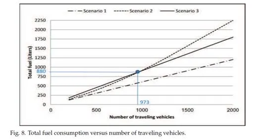
It is obvious that Hwy 1 is the best choice in terms of distance, travel time, fuel consumption, and emissions. However, if an accident happened on Hwy 1, it might not be the best choice for the drivers. Focusing on the fuel consumption, it is assumed that each vehicle has a navigation system that advises drivers on route selection based on minimizing trip fuel consumption. Figure 8 shows the impact of increasing the number of traveling vehicles on the total vehicles’ fuel consumption. It is clear and expected that Scenario 1 is most economical. Consequently, the navigation system will advise the driver to travel on Hwy 1. However, if an accident happened on Hwy 1, a significant amount of fuel can be wasted due to stop-and-go conditions and congestion. It can be noticed from Figure 8 that Scenario 2 is more economical than Scenario 3 in light traffic density. Conversely, Scenario 3 becomes more economical than Scenario 2 with increasing traffic density.
Since navigation systems are not aware of the sudden events (e.g., accidents), vehicle-to-vehicle communications will be needed. With a focus on geocast, two main points have to be considered in order to design an economical protocol:
Geocast region The warning message has to be delivered to the region so that drivers can find a new path to avoid congestion.
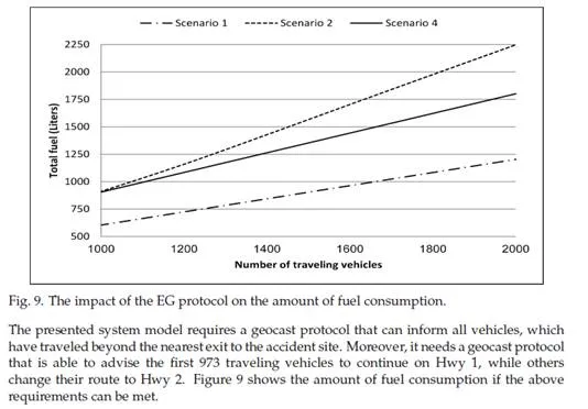
Delivered Message A warning message will be issued once an accident occurs in order to alert nearby vehicles. Based on the results shown in Figure 8, not all alert routes (i.e. routes with accident “Scenario 2″) consume more fuel than no alert routes “Scenario 3″. Therefore, we need to define when the status of the most economical route will change from Hwy 1 to Hwy 2 (this depends on the traffic density). Then, find a way to inform the drivers.
Discussions
The important issues that have to be taken into account in designing an economical geocast protocol in this model are as follows:
Calculating the Desirable Number of Traveling Vehicles on Hwy 1: The desirable number of traveling vehicles is 973 in this study. This number was obtained from the simulator. However, research is needed to be done to estimate this number. This information can be used in designing communication applications. Consequently, the geocast packet will contain this information when a geocast is performed. In conclusion, ITS applications and tools should be able to calculate this kind of information and inject it to the geocast packet.
Traffic Density versus Fuel Consumption: In many cases the shortest path in terms of time or distance will also be the minimum fuel consumption. However, this is not true in several cases which increase traffic. For instance, congestion will start if an accident happened. In this case, stop-and-go conditions will occur; thus, more fuel will be consumed. Therefore, changing to another path even if it is longer is preferred. In addition, it is important to point that in some cases, an accident might happen on a highway, but the vehicles do not need to change the path since it is still the best in terms of fuel consumption. This issue depends on the traffic density.
Defining the region of interest: In this work, the target region is 2 km beyond the nearest exit. However, the idea of region of interest needs to be investigated. In references (Rezaei et al., 2009a;b; Rezaei, 2009c), the region of interest has been determined base on the type of warning messages and traffic density. Moreover, two metrics have been defined to
City environment
This example illustrates the benefit of transmitting the traffic light signal information to vehicles for CO2 emission reduction. Simulation results demonstrate that vehicle CO2 emission will be reduced if such an environmentally friendly geocast (EFG )protocol is used.
System model
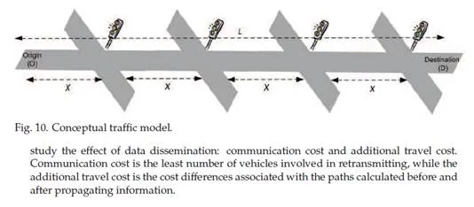
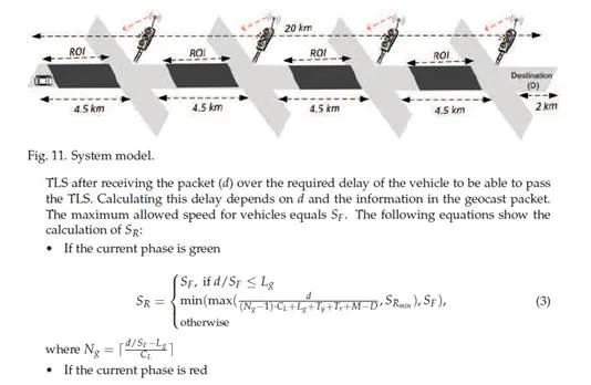
Traffic Model: As shown in Fig. 10, a vehicle’s trip initiates from the Origin (O) to the Destination (D). A street segment with length L and N-lanes has been considered. This segment has four static Traffic Light Signals (TLSs). The distance between each TLS and the following one is X. Each TLS has three phases: green, yellow, and red. The phase duration is Tg , Ty , and Tr for green, yellow, and red, respectively. The free-flow speed of the street is SF m/s.
Fuel Consumption and Emission Model: Similar to the example in Section 5.1, the VT-Micro model has been used in this example due to its simplicity and high accuracy.
Communication Model: Assume that TLSs and the traveling vehicle are equipped with an On-Board Unit (OBU). The assumption that the OBU is equipped with a (short range) wireless communication device is considered. In addition to OBU, the traveling vehicle is equipped with an Application Unit (AU). It is assumed that the AU is equipped with position data and map (e.g., GPS). Therefore, the vehicle knows its location and the location of TLSs. The TLSs are the transmitters, while the destination is addressed as all vehicles in a Region of Interest (ROI).
Each TLS sends a geocast packet within a transmission range which is equal to the ROI. This packet is directed to vehicles approaching the signal. The geocast packet is considered to contain three types of information:
1. Type of the current phase (either green “g”, yellow “y”, or red “r”);
2. Number of seconds to switch from the current phase (Lg , Ly , or Lr );
3. Traffic light schedule, which includes the full green, yellow, and red phase time (Tg , Ty , and Tr ).
With these information, the vehicle calculates a recommended speed (SR ) for the driver to avoid stopping at the TLS. SR can be calculated as the distance between the vehicle and the
Simulation study and discussions
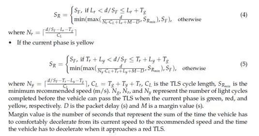
The length of the street and the distances between the TLSs are shown in Figure 11. The street has one lane and is in one direction. The ROI is changeable from 0.5 to 4.5 km in increments of 0.5. The rest of the simulation parameters are specified in Table 5.
The simulator used is INTEGRATION. In this example, the total vehicle’s CO2 emission have been computed at different ROIs. We assume that the TLSs send a packet at the moment when the vehicle entered the ROI. In this case, the distance between the vehicle and the TLS is almost equal to the ROI.
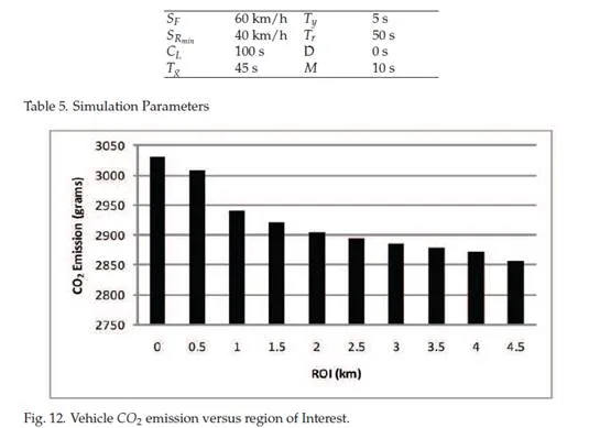
Figure 12 shows the impact of the length of the ROI on the amount of the vehicle’s CO2 emission. With a large ROI, the vehicle will have more time to avoid stops and accelerations. Therefore, the amount of the vehicle’s CO2 emission decreases with increasing ROI as shown in the figure.
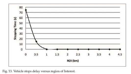
Figure 13 shows how stopping time decreases as ROI increases for a vehicle that travels from O to D. It is clear that in the absence of communication between the TLSs and the vehicle, the vehicle will stop for around 75 seconds. This time would be shortened if the idea of vehicular networks is applied. It can be seen that the vehicle will keep passing all TLSs without stopping when the geocast packet can cover at least 1 km ahead of each TLS.
Consider that the vehicle travels at the free-flow speed if it is out of the ROI. After receiving the geocast packet from the TLS, the vehicle will recommend to the driver the environmentally friendly speed as in Eqs. 3, 4, and 5. The goal of calculating this speed is to have the vehicle avoid unnecessary stops, useless acceleration and high speed.
The vehicle may avoid a stop by adapting its speed to (SR ), such that SRmin ≤ SR ≤ SF . The vehicle will adjust its speed to SRmin in order to avoid useless high speed if it is impossible for the vehicle to avoid stopping. The last goal is to alleviate vehicle accelerations. This can be
achieved by calculating the SR as the maximum possible speed for the vehicle to pass the TLS with no stops. As a result, after passing the TLS, the vehicle will return to the free-flow speed with low acceleration.
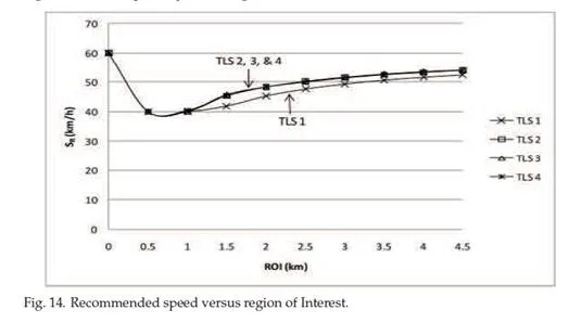
Figure 14 shows the impact of the increase of the ROI on the SR . With no vehicular network, the vehicle is not aware of the TLS information; therefore, it travels at the maximum allowed speed. At ROI = 0.5 km, the vehicle will realize that stopping will happen. Consequently, the recommended speed is reduced to SRmin . After that, the SR will increase with increasing ROI.
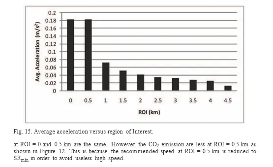
Figure 15 shows the benefit of increasing the ROI to alleviate average vehicle acceleration. At
ROI = 0 and 0.5 km, the vehicle stops at each TLS. Therefore, the average vehicle acceleration
Conclusions
This chapter is to show the impact of vehicular networks on vehicle fuel consumption and CO2 emissions. This chapter also aims to motivate researchers working in the field of communication to design EEFG protocols, and demonstrate the ability to integrate fuel consumption and emission models with vehicular networks. The first example was in a highway environment with the fuel consumption as the performance metric. This example illustrates the necessity of sending information to vehicles in order for drivers to choose an appropriate path to a target to minimize fuel consumption. Simulation results demonstrate that significant amounts of fuel will be saved if such an EG protocol is used. The second example was in a city environment with considering the CO2 emission as the performance metric. This example illustrates the benefit of transmitting the traffic light signal information to vehicles for fuel consumption and emission reduction. Simulation results demonstrate that vehicle fuel consumption and CO2 emissions will be reduced if such an environmentally friendly geocast protocol is used.