Congestion has grown over the past two decades making the travel time highly unreliable. The Federal Highway Administration (FHWA), US Department of Transportation (USDOT) indicated travel time as an important index to measure congestion. Frequent but stochastic, irregular delays increase the challenge for people to plan their journey – e.g. when to depart from the origin, which mode(s) and route(s) to use so the on-time arrival at the destination can be ensured. In addition to average travel time, the reliability of travel time has been deemed as an index for quantifying the effects of congestion, which can be applied to the areas of transportation system planning, management and operations as well as network modeling. Travel time reliability has been classified into two categories: probability of a non-failure over time and variability of travel time (Elefteriadou and Cui, 2005).
The variability of travel time plays an important role in the Intelligent Transportation Systems (ITS) applications. According to the Safe, Accountable Flexible, Efficient Transportation Equity Act: A Legacy for Users (SAFETEA-LU) Reporting and Evaluation Guidelines, travel time variability indicates the variability of travel time from an origin to a destination in the transportation network, including any modal transfers or en-route stops. This measure can readily be applied to intermodal freight (goods) movement as well as personal travel. Reducing the variability of travel time increases predictability for which important planning and scheduling decisions can be made by travelers or transportation service suppliers. In the advent of ITS, the incident impact, such as delay, may be reduced via disseminating real-time traffic information, such as the travel time and its variability. Travel time variability has been extensively applied in transportation network models and algorithms for finding optimal paths (Zhou 2008). The recent ITS applications highlighted the needs for better models in handling behavioral processes involved in travel decisions. It was indicated that travel time variability has affected the travelers’ route choice (Avineri and Prashker, 2002). The relationship between the estimated travel time reliability and the frequency of probe vehicles was investigated by Yamamoto et al (2006). It was found that the accuracy of travel time estimates using low-frequency floating car data (FCD) appears little different from high-frequency data.
Recker et al. (2005) indicated that travel time variability is increasingly being recognized as a major factor influencing travel decisions and, consequently, is an important performance measure in transportation management. An analysis of segment travel time variability was conducted, in which a GIS traffic database was applied. Standard deviation and normalized standard deviation were used as measures of variability. Brownstone et al. (2005) indicated that the most important facor is the “value of time” (VOT), i.e. the marginal rate of travel time substitution for money in a travelers’ indirect utility function. Another factor is the value of reliability (VOR), which measures travelers’ willingness to pay for reductions in the day-to-day variability of travel times facing a particular type of trip. Bartin and Ozbay (2006) identified the optimal routes for real-time traveler information on New Jersey Turnpike, which maximizes the benefit of motorists. The variance of travel times within a time period over consecutive days was employed as an indicator of uncertainty. With the concept of multi-objective approach, Sen and Pillai (2001) developed a mean-variance model for optimizing route guidance problems. The tradeoff between the mean and variability of travel time was discussed. For improving decision reliability, Lu et al. (2005) developed a statistic method to analyze the moments and central moments of historic travel time data, which provided quantitative information on the variability and asymmetry of travel time. Palma et al. (2005) conducted a study in Paris to determine the route choice behavior when travel time is uncertain. Both the mean and variability of travel time were considered.
Objective
The objective of this chapter is to investigate the measurement of travel time variability and reliability with FCD. Considering the Variability of Travel Time (VTT) as a component of mobility performance metrics, this chapter discusses technologies and methodology applied to collect, process and analyze the travel time data. To analyze the impact of travel time due to non-recurring congestion, three case studies on selected highways were conducted. As defined in a report titled “Traffic Congestion and Reliability: Trends and Advanced Strategies for Congestion Mitigation” (FHWA, 2005), the travel time reliability was deemed as how much travel time varies over the course of time. The variation in travel times from one day to the next is due to the fact that underlying conditions (such as vehicle composition, weather conditions) vary widely. Seven sources of congestion are identified, including physical bottlenecks (“capacity”), traffic incidents, work zones, weather, traffic control devices, special events, and fluctuations in normal traffic condition, which contribute to total congestion and conspire to produce biased travel time estimates.
Statistical indices
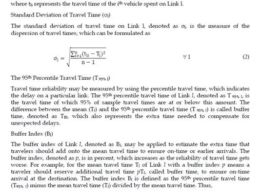
To estimate travel time variability with FCD, statistical formulas for generating suitable reliability indicators, such as mean, standard deviation, the 95th percentile travel time, and buffer index, etc are utilized.
Mean Travel Time (Tl)
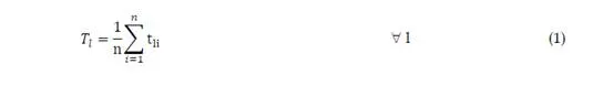
The mean travel time, denoted as Tl, is equal to the sum of the travel time collected by a number of floating cars, denoted as n, traveling on Link l. Thus,
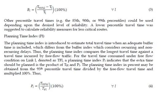
The planning time index is useful since it can be directly compared to the travel time index (a measure of average congestion) on similar numeric scales. Note that the buffer index represents the additional percent of travel time that is necessary above the mean travel time, whereas the planning time index represents the total travel time that is necessary. Thus, the buffer index was used to be applied to estimate non-recurring delays.
Various travel time reliability measures have been discussed in previous studies, but only few of them are effective in terms of communication with road users and general public. Buffer index (BI) and planning time index (PI) are ones of the most effective methods in measuring travel time reliability (FHWA). Other statistical measures, such as standard deviation and coefficient of variation, have been used to quantify travel time reliability, but they are not easy for a non-technical audience to understand and would be less-effective communication tools.
Case studies
With FCD, three case studies are conducted for investigating the variability of travel time, including (1) analysis of temporal and spatial travel times, (2) evaluation of adverse weather impact to travel time variability and reliability, and (3) investigating travel time variability in a freeway network.
Case study I – Analysis of temporal and spatial travel times
The first set of the travel time FCD were collected to assess the impacts of special events, traffic control devices and bottleneck on travel time variability. The travel time data were collected by floating cars with GPS-based sensors traveling on the segments of I-295 and the New Jersey Turnpike (NJTP) from 10:00 to 19:00 on three different Sundays: May 24, June 7, and July 19 in 2009. On an hourly basis starting at 10:00, two floating cars were dispatched simultaneously, one heading for the I-295 segment and the other heading for the NJTP segment. To investigate the travel time variability and congestion of the studied segments, the collected data were analyzed on a link (e.g., links 1, 2, and 3) and a path (e.g., from Node1 to Node 4) basis, as shown in Figure 1. The geographic information of each route
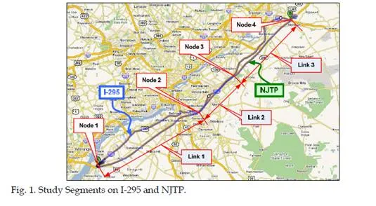
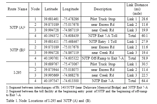
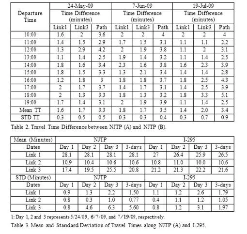
Since tolls are collected at the entrances and exits of NJTP, the travel times of two segments [e.g., NJTP (A) and NJTP (B)] were prepared and estimated. NJTP (A) includes the toll payment process and starts from interchange Rt. 140/NJTP and ends at NJTP Exit 7-A. To estimate the travel time excluding delays at toll plazas, NJTP (B) starts right after the first toll facility on the NJTP and ends at the beginning of the off ramp to Exit 7-A. The impact of tolls on the travel time was estimated by comparing the travel time difference between these segments as shown in Table 2. It can be easily observed that the first toll facility contributes
1.6 minutes average delay and the second toll facility provides a slightly longer average delay as 1.8 minutes. The standard deviation to the travel time is 0.3 minute for the first toll and 0.5 minute for the second toll based on a 9-hour observation period from 10:00 to 19:00.
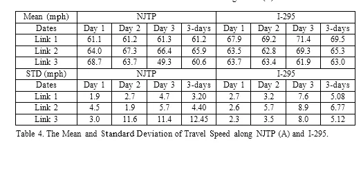
The link- based travel times are collected by probe vehicles dispatched at each hour on survey days. Table 3 summarizes the mean travel times and the associated standard deviations. The speeds are also estimated based on the travel time and the corresponding link distance, and the statistical results are summarized in Table 4. It can be observed in Table 3 that less travel time was consumed on Link 1 of I-295 than that of NJTP with standard deviation to the mean. For Link 2, the mean travel times of I-295 and NJTP were the same, but the standard deviations to the means of NJTP for all travel time data on the three survey days were consistently less than that of I-295, which indicates that Link 2 of NJTP is more reliable than that of I-295. For Link 3, the mean travel time of NJTP was 20.8 minutes, slightly shorter than that of I-295 (e.g. 21.6 minutes). The standard deviation of travel time of NJTP was significantly higher than that of I-295, was incurred by congestion on NJTP (See Figures 2 and 3).
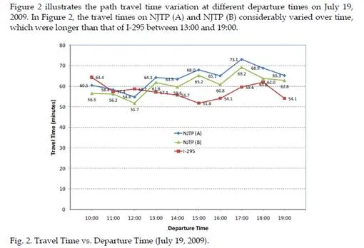
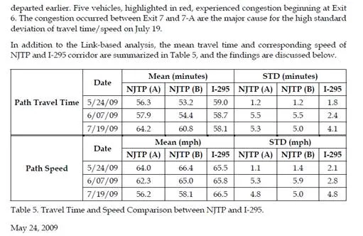
The mean travel time of NJTP (A) was 56.3 minutes, which was shorter than that of the I-295
segment (59.0 minutes). The standard deviation of the mean travel time of NJTP (A) was 1.2 minutes, which was less than that of I-295 (1.8 minutes). Thus, the travel time of NJTP (A) segment was shorter and more reliable than that of the I-295 segment on 5/24/09. Travelers would be recommended to use NJTP instead of I-295 because of shorter and more reliable travel time.
June 7, 2009
The mean travel time on NJTP (A) was 57.9 minutes and the standard deviation of the mean was 5.5 minutes. On the other hand, the mean travel time on I-295 was 58.7 minutes, which was longer than that of NJTP (A); however, the standard deviation to the mean was 2.4 minutes, which was significantly less than that of NJTP (A). Thus, using NJTP (A) was not always quicker than I-295, and the reliability of travel time of the NJTP was less than that of I-295 on 6/7/09. Travelers would have been better using I-295 if they departed between
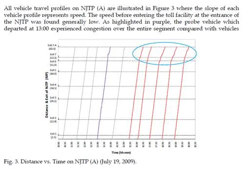
14:00 and 15:00, as they would have avoided congestion between Exits 7 and 7-A. July 19, 2009
The mean travel time on NJTP (A) was 64.2 minutes and the standard deviation to the mean was 5.3 minutes. The mean travel time on I-295 was 58.1 minutes, shorter than that of NJTP (A), and the standard deviation to the mean was 4.1 minutes. It was found that using I-295 was quicker than NJTP (A) at the departure time of 13:00 through 19:00, and the reliability of travel time of I-295 was more than that of NJTP (A). Travelers would have been better using I-
295 if they departed between 15:00 and 19:00, as they avoided congestion beginning at Exit 6.
Based on the mean speed and standard deviation, the travel time of these two parallel freeways were compared to identify the bottlenecks, evaluate their reliabilities and propose strategies to address congestion problems. For example, the observed congestion on NJTP (A) was found between Exits 6 and 7-A. Thus, it is recommended to use Dynamic Message Sign (DMS) at interchange 4 and Highway Advisory Radio (HAR) to inform drivers of congestion ahead.
Case study II – Analysis of adverse weather impact to travel time variability and reliability
The second set of travel time data intended for assessing weather impact were obtained through TRANSMIT system (TRANSCOM’s System for Managing Incidents & Traffic). TRANSMIT uses vehicles equipped with electronic toll-collection tags (EZ-Pass) detected by roadside readers to approximate real-time travel time. The travel time data between
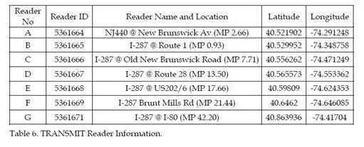
1/29/2008 and 2/29/2008 were collected on a 40-mile segment of the Interstate I-287 consisting of six links divided by seven TRANSMIT readers. The weather information was collected from a website (http://www.wunderground.com/US/NJ) managed by a weather data provider. Adverse weather conditions, such as rain, fog and snow, occasionally cause delay on roadways. The variation of travel times due to adverse weather should be concerned by agencies managing traffic operations and evaluating network-wide mobility. The measured variability and reliability indices discussed earlier will also help in trip planning under different weather conditions. The travel time data were collected by the TRANSMIT readers under three weather conditions, normal (dry), rain, and snow, during the AM peak period (6:00 AM ~ 9:00 AM) on weekdays. The mean and standard deviation of travel time, the 95th percentile travel time and buffer index were analyzed to quantify the impact of adverse weather to traffic conditions.
The day-to-day and within-day travel time were collected between 1/29/2008 and
2/29/2008. The start and end mile-posts (MP) and geo-coordinates of the TRANSMIT
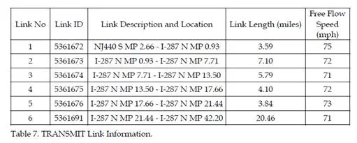
readers are summarized in Table 6. Link 6 has very long stretch, which is 20 miles from Exit
21 to Exit 41 on I-287. In Table 7, the link specific data are summarized, which includes link ID number and length. The mean, the 95th percentile, and the standard deviation of travel time as well as buffer index of each link are estimated by the equations discussed earlier in this paper.
Day-to-day Travel Time Variation
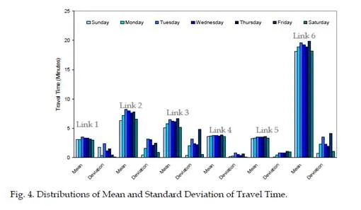
Figure 4 indicates the mean and standard deviation of travel time on each link over different
days. Results, in general, show that the mean travel times on Tuesdays and Fridays are relatively higher than other days. The greatest travel time happened on Link 6 which is not surprising because the link distance is much longer than others. The greatest standard deviation of travel time was observed on Link 3 on Fridays. It is worth noting that the length of Link 3 is 5.79 mile, and the mean travel time was 6 minutes, but the standard deviation of travel time was 5 minutes. The ratio of the standard deviation of travel time to the mean travel time of Link 3 on Fridays was extremely high.
The spatial and temporal distributions of the 95th percentile travel time of Link 6 are analyzed and shown in Figure 5, where the day-to-day travel time on each link seemed following a trend of mean travel time distributions shown in Figure 4. The motorists traveling on Tuesdays and Fridays generally suffered more congestion as well as the travel time uncertainty.
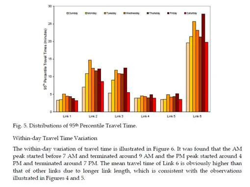
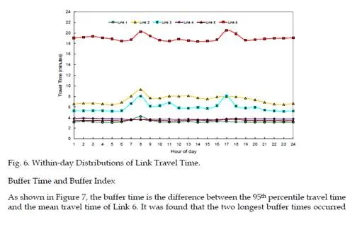
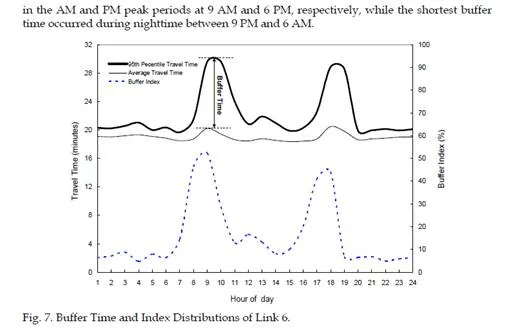
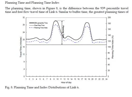
Link 6 occurred in the AM and PM peaks. As indicated in the above sections, the planning time index compares the worst case travel time to the travel time consumed under free-flow traffic condition.
Considering the whole studied I-287 segment, the travel time increased 10% and 60% under rain and snow, respectively. Moreover, it was found that the impact of adverse weather to traffic operation was much more significant during the peak periods than that during the off-peak periods.
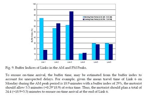
The buffer Index of each link was calculated using Eq. 3 based on data collected under normal weather condition (18 days with dry pavement). To well plan for a journey, it is critical to know the buffer index, especially during the peak periods. In this study, the buffer indices of the AM and PM peaks were illustrated in Figure 9. In the AM peak, the worst buffer index was found on Link 1 with 75% while the best one was on Link 4 with 11%. In the PM peak, the worst buffer index was on Link 3 with 86%, while the best one was on Link
4 with 12%.
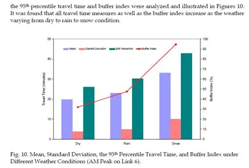
Based on the buffer index shown in Figure 10, the variation (standard deviation) of travel time increased due to the weather condition varied from dry to rain and rain to snow. In addition, the buffer index also increased from 29%, 45%, to 94%. If a motorist needs to travel on Link 6 under rain, 16% (45%-29%) of extra time of the mean travel time under dry condition should be expected. However, under a snow day, the addition of 65% (94%-29%) of the mean travel time should be expected.
It was found that adverse weather, such as rain and snow, had significant impact on delay and associated travel time variability when compared with traffic operation under dry condition. Considering the whole studied I-287 segment, the travel time increased 10% and
60% under rain and snow, respectively. Moreover, it was found that the impact of adverse weather to traffic operation was much more significant during the peak periods than that during the off-peak periods.
Case study III – Investigating travel time variability in a freeway network
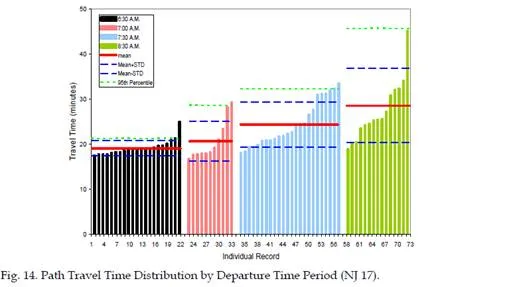
The third set of travel time data were used to analyze the travel time reliability under recurring and non-recurring traffic congestion. Travel time collection was conducted on the segments of fifteen New Jersey highways including: Routes US 1, NJ 4, US 9, NJ 17, US 22, NJ 24, NJ 29, NJ 42, US 46, NJ 70, NJ 73, I-76, I-78, I-80, I-280, and I-287 during the AM peak hours on weekdays between October 8, 2007 and April 21, 2008 through the use of Co- Pilot™ GPS navigation devices. In order to identify the link- and path-based travel time distributions of NJ 17, the following analysis was conducted:
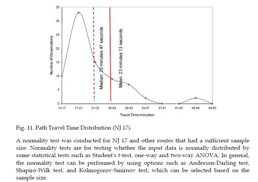
The frequency of the route travel time for the entire departure time period from 6:15 to 8:15
AM is shown in Figure 11. The path travel time data were classified into four-minute time intervals, and the distribution is a shifted log-normal distribution. The Y- axis is intercepted at the free flow travel time then it is followed by a bell shape and then it has a long tail of path travel time observations that reflect the delays experienced due to various traffic flow conditions such as increases in demand and incidents.
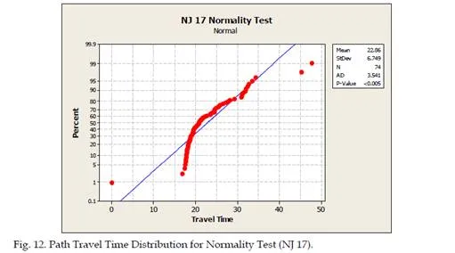
In order to determine whether a travel time distribution is normal or log-normal, hypothesis test was applied. The smaller the p-value, the more strongly the test rejects the null hypothesis. A p-value of 0.05 or less rejects the null hypothesis. The statistical statement for the normality test is
Null Hypothesis( H0): The route travel time distribution for NJ 17 follows the Normal distribution
Alternative Hypothesis (Ha): The route travel time distribution for NJ 17 has a different distribution than the Normal.
Figure 12 indicates that the null hypothesis – the route travel time distribution is normal – is rejected as quite a few observations fall away from the line. The p-value (<0.005) of less than
0.05 confirms the visual observation of the normality test.
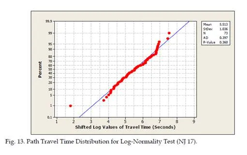
A Log-Normality test for the path travel time was also conducted. The collected path travel time was converted log-value and the shortest travel time was subtracted from each observation since the travel time distribution seems to fit a shifted log-normal distribution. Figure 13 indicates that the null hypothesis (e.g. the route travel time distribution is log-normal) is not rejected as only a few observations fall away from the line. The corresponding p-value (0.36) of greater than 0.05 confirms the visual observation of the log-normality test.
Conclusions
The chapter discussed methods to estimate the variability and reliability of travel times. Floating cars with GPS devices were proven as an applicable tool to collect travel time. The travel time variability and reliability were successfully assessed based on the mean travel time, the 95th percentile travel time, travel time index, buffer index, and planning time index, etc. The impact of stochastic factors on the corridor travel time was identified for the traffic management by public agencies. The GPS-based link/path travel time data could be used for producing the Measures Of Effectiveness (MOEs) thereby assisting real-time traffic control (e.g. signal timing) and traveler information (e.g. traffic diversion and travel planning), and transportation planning (e.g. infrastructure and traffic management strategies).
Many public transportation agencies have been focusing on enhancing the capability of data collection, processing, analysis and management to generate reliable estimates. In most cases, however, travel time data are available for relatively few corridors in a state and sometimes suffered by limited sample sizes. It is desirable to collect vast data in good quality and develop a cost-effective method to measure travel time variability and reliability that will be of interests of practitioners in measuring and predicting the transportation network performance. This study investigates the variability of travel time measurements based on broad traffic environments and their impacts on the ITS applications. It is recommended that the developed methodology can be used to produce link- and path-based travel time distributions associated with the Buffer Indices as performance measures to aid planners and engineers in making decisions of highway improvements and transportation management to reduce delays while improving reliability.