
A driver sees a traffic signal change, a pedestrian step from between parked cars, or the line of vehicles ahead begin to slow. In that short moment, the car does not stop instantly. It continues to travel while the driver reacts, while the brakes build force, and while the tyres convert motion into heat against the road.
That gap between noticing a hazard and coming to rest is the vehicle’s stopping distance. It is one of the most practical calculations in automobile engineering because it connects physics to real design decisions: brake sizing, tyre selection, road layout, driver-assistance calibration, and safe speed choice.
Speed changes the result more sharply than intuition suggests. Doubling speed doubles the distance travelled during a fixed reaction time, but the ideal braking distance rises by roughly four times. This is why a modest increase in speed can leave much less room for error.
A braking-distance calculation is therefore not a promise that every vehicle will stop at one exact point. It is a structured estimate based on assumptions. Understanding those assumptions is as valuable as using the equation.
🛑 What Braking Distance Actually Means
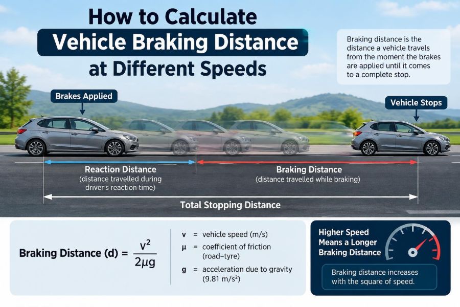
Braking distance is the distance travelled from the moment effective braking begins until the vehicle reaches zero speed. It does not include the distance covered while the driver perceives danger and moves a foot to the brake pedal.
This distinction matters in engineering and road safety discussions. A vehicle may have excellent brakes yet still travel a considerable distance before braking starts if the driver is distracted or a control system has not detected the hazard.
📏 Stopping Distance Has Three Parts
In everyday use, “braking distance” often means the entire distance needed to stop. Technically, total stopping distance can be separated into three stages:
- Perception distance: distance travelled while recognizing a hazard.
- Reaction distance: distance travelled while deciding and applying the brake.
- Braking distance: distance travelled after braking force acts on the vehicle.
For a simplified driver model, perception and reaction are often combined into one reaction time. Mechanical brake response can also add a small delay, particularly in heavy vehicles or complex pneumatic systems.
⚙️ The Core Physics Behind the Calculation
A moving vehicle has kinetic energy. For a vehicle of mass m travelling at speed v, kinetic energy is:
KE = 1/2 mv²To stop, the brake system and tyre-road contact must remove this energy. Most is converted to heat in brake discs or drums, pads or shoes, tyres, and the road surface. Some is dissipated through aerodynamic drag and rolling resistance.
The squared speed term is the critical feature. At twice the speed, the vehicle carries four times the kinetic energy for the same mass.
🧮 The Basic Braking-Distance Formula
On a level road, assuming approximately constant deceleration, braking distance can be calculated as:
d = v² / (2a)Here, d is braking distance in metres, v is initial speed in metres per second, and a is the magnitude of deceleration in metres per second squared. Deceleration is written as a positive magnitude in this formula, even though acceleration is physically negative during braking.
This model is especially useful for comparing speeds or estimating the effect of a change in available grip. It is an idealization, not a substitute for measured stopping tests.
🔁 Converting Road Speeds into SI Units
Engineers use metres per second because the standard kinematic equations are expressed in SI units. Convert kilometres per hour by dividing by 3.6:
v (m/s) = speed (km/h) / 3.6For miles per hour, multiply by approximately 0.447 to obtain metres per second. Do not place km/h directly into the basic formula; doing so produces a severely incorrect result.
For example, 60 km/h is 16.67 m/s, not 60 m/s. That conversion alone changes the squared-speed calculation dramatically.
🛞 Estimating Deceleration from Tyre-Road Friction
When tyre-road grip limits braking, deceleration can be estimated with the friction coefficient μ:
a = μgIn this expression, g is gravitational acceleration, approximately 9.81 m/s². Combining it with the basic braking formula gives:
d = v² / (2μg)The coefficient μ is not a fixed property of “dry road” or “wet road.” It changes with tyre compound, tread condition, road texture, temperature, water depth, contamination, load transfer, and whether the tyre is rolling near its optimum slip level.
📉 Why Speed Has a Squared Effect
Suppose road and tyre conditions allow the same deceleration at two speeds. If speed doubles, v² becomes four times larger, so braking distance becomes four times larger.
This is not merely a mathematical curiosity. A driver travelling at 80 km/h instead of 40 km/h has twice the speed but approximately four times the ideal braking distance, before reaction distance is added. Aerodynamic drag can help slightly at higher speeds, but it does not remove this dominant relationship in normal road braking.
🧾 Worked Example: Braking from 50 km/h
Consider a hypothetical car on a level, dry road. Let its assumed achievable deceleration be 7.0 m/s². First convert 50 km/h:
v = 50 / 3.6 = 13.89 m/sThen apply the formula:
d = 13.89² / (2 × 7.0) = 13.8 m approximatelyUnder these assumptions, the braking distance is about 14 m. This excludes driver reaction distance, and actual test results could differ because the assumed deceleration may not match the actual car, tyres, surface, or brake condition.
🚘 Comparing Distances at Different Speeds
The following hypothetical values use a constant deceleration of 7.0 m/s² on a level surface. They illustrate the speed relationship rather than predict every vehicle’s real-world performance.
| Initial speed | Speed in m/s | Calculated braking distance |
|---|---|---|
| 30 km/h | 8.33 | About 5 m |
| 50 km/h | 13.89 | About 14 m |
| 80 km/h | 22.22 | About 35 m |
| 100 km/h | 27.78 | About 55 m |
| 120 km/h | 33.33 | About 79 m |
The 100 km/h value is roughly four times the 50 km/h value, consistent with the squared-speed relationship.
⏱️ Calculating Reaction Distance
Reaction distance uses a simpler relationship:
dreaction = v × tSpeed is in metres per second and t is reaction time in seconds. At 50 km/h, a vehicle travels about 13.9 m in one second. At 100 km/h, it travels about 27.8 m in one second.
Reaction time varies substantially with alertness, visibility, expectation, fatigue, distraction, impairment, and the complexity of the situation. A fixed value is useful for an estimate, but should never be mistaken for a universal human constant.
➕ Building a Total Stopping-Distance Estimate
A practical simplified model is:
total stopping distance = reaction distance + braking distanceFor the earlier 50 km/h example, assume a 1.5-second reaction time. Reaction distance is 13.89 × 1.5, or about 20.8 m. Adding the estimated 13.8 m braking distance gives a total of about 34.6 m.
At 100 km/h with the same assumptions, reaction distance is about 41.7 m and braking distance about 55.1 m. Total distance becomes nearly 97 m. Both components grow with speed, but braking distance grows faster.
🌧️ Wet Roads Reduce Available Grip
Water can separate parts of the tyre tread from the road texture and reduce the friction available for braking. If the available friction coefficient falls, deceleration falls, and the calculated braking distance rises.
The effect is not identical in every shower. Light rain after a dry period can mix with surface contaminants; standing water may create a much larger problem; good tread and a textured surface can improve water evacuation. The safe engineering conclusion is to use a lower assumed deceleration whenever grip is uncertain.
❄️ Snow, Ice, and the Limits of Simple Estimates
Snow and ice can reduce tyre-road friction far more than ordinary wet pavement. The same formula still describes the direction of change, but selecting one friction coefficient becomes difficult because the surface can vary over a few metres.
A polished icy patch, compacted snow, loose snow, grit, temperature, and winter tyre design can all alter the result. Under such conditions, large following gaps and lower speeds are more reliable safety measures than confidence in a single calculated distance.
🛞 Tyres Are the Final Link to the Road
Brake torque reaches the road only through four contact patches, each roughly tyre-sized rather than vehicle-sized. Tyre condition therefore influences stopping performance as directly as many brake components do.
- Worn tread reduces the ability to clear water and can worsen wet braking.
- Incorrect inflation changes the contact-patch behaviour and tyre temperature.
- Age, damage, and unsuitable compound reduce predictable grip.
- Tyres on the same vehicle should be compatible in size, construction, and intended use.
New brakes cannot compensate fully for tyres that cannot generate adequate longitudinal force.
🧲 How Brake Force Produces Deceleration
Pressing the pedal creates hydraulic pressure in most passenger cars. Caliper pistons clamp pads onto brake discs, or wheel cylinders press shoes against drums. Friction at these components creates brake torque at each wheel.
That torque slows wheel rotation. At the tyre contact patch, the road applies a rearward force to the vehicle, reducing its forward speed. If demanded brake torque exceeds available tyre grip, the wheel tends to lock rather than deliver greater deceleration.
🧠 ABS Helps Preserve Control, Not Create Unlimited Grip
An anti-lock braking system, or ABS, monitors wheel speeds and modulates brake pressure when it detects impending wheel lock. Its central purpose is to keep tyres near a useful slip range so the driver can retain steering control.
On many surfaces, ABS can also support strong braking by avoiding prolonged lock-up. However, it cannot create friction where little exists. Surface irregularity, loose material, tyres, and vehicle condition still determine the available braking force.
⚖️ Weight Transfer Changes Front and Rear Loads
During hard braking, the vehicle’s centre of mass continues moving forward, transferring load toward the front axle. The front tyres are pressed harder into the road while the rear tyres carry less vertical load.
This is why front brakes usually provide more braking force than rear brakes in passenger vehicles. Brake proportioning, electronic brake-force distribution, suspension geometry, wheelbase, and centre-of-gravity height all affect how the braking demand should be shared.
🏋️ Vehicle Mass: Important, but Not in the Simplest Model
The basic friction-limited formula d = v²/(2μg) contains no mass term. In an ideal case, a heavier vehicle has more kinetic energy, but it also presses its tyres harder onto the road by the same proportion, so mass cancels.
Real vehicles are not perfectly ideal. Tyres are load-sensitive, brakes can heat differently, payload distribution changes axle loads, and heavy vehicles may have different braking hardware. Mass therefore matters greatly in real design and testing even though it disappears from the simplest equation.
🔥 Brake Fade and Repeated High-Energy Stops
One emergency stop may be very different from a sequence of long downhill or high-speed stops. As discs, pads, drums, brake fluid, and other components heat up, the system may lose some ability to produce consistent braking torque.
Brake fade is a reduction in braking effectiveness caused by overheating-related mechanisms. These may include changes in friction material behaviour, overheating of drum components, or fluid boiling in severe cases. Proper maintenance, correctly specified components, and lower gear selection on descents help manage heat.
⛰️ Road Gradient Adds or Removes Braking Demand
On a downhill, gravity has a component pulling the vehicle forward. On an uphill, gravity helps slow it. A more complete slope calculation can be written approximately as:
a = μg cos(θ) + g sin(θ)For downhill travel, the slope term acts against deceleration, so the sign must be handled carefully according to the chosen coordinate direction. On small gradients, the effect may seem modest, but it becomes meaningful at higher speeds, on long descents, or when grip is already low.
🌬️ Aerodynamic Drag Is Present but Usually Secondary
Air resistance increases strongly with speed and acts opposite to motion, so it assists braking. Rolling resistance also removes a small amount of energy. These effects mean a real deceleration trace is not always perfectly constant.
For ordinary emergency-braking estimates, tyre-road force is usually the main factor and the constant-deceleration model remains useful. For detailed vehicle simulation, high-speed testing, or performance development, engineers model aerodynamic drag, rolling resistance, rotating inertia, and changing brake force explicitly.
📊 Stopping Tests Use Measured Data
Vehicle engineers do not rely only on equations. They instrument vehicles to measure speed, deceleration, pedal force, wheel speeds, brake temperatures, stopping distance, yaw behaviour, and surface conditions.
Repeated tests reveal variation that a one-line formula cannot show. A test result is meaningful only with context: initial speed, tyre specification, tyre pressure, road surface, vehicle loading, ambient conditions, brake state, and whether ABS was active all influence interpretation.
🧭 Deceleration, g-Force, and What Drivers Feel
Deceleration is sometimes described as a fraction of g. A deceleration of 0.7 g means approximately 0.7 × 9.81 m/s², or about 6.9 m/s².
Drivers feel this as a strong forward load against the restraint system. A high deceleration number may indicate effective grip and braking, but it is not sufficient by itself: stability, steering control, repeatability, passenger comfort, and surface consistency also matter.
🧰 A Practical Calculation Workflow
For a transparent first estimate, use a consistent process rather than choosing a distance by intuition:
- State the initial speed and convert it to m/s.
- Describe the road, tyres, vehicle loading, and gradient.
- Select a cautious assumed deceleration or friction coefficient.
- Calculate braking distance using
d = v²/(2a). - Choose and state a reaction-time assumption.
- Calculate reaction distance using
d = vt. - Add the components, then communicate uncertainty clearly.
The stated assumptions are part of the answer. Without them, a numerical stopping distance can appear more precise than it really is.
🧪 Example: Comparing 60 km/h and 90 km/h
Assume a level surface and a deceleration of 6.5 m/s². At 60 km/h, speed is 16.67 m/s, giving a braking distance of about 21.4 m. At 90 km/h, speed is 25.0 m/s, giving about 48.1 m.
The speed rose by 50%, from 60 to 90 km/h, but braking distance increased by about 125%. If the same 1.5-second reaction time is assumed, reaction distance rises from 25 m to 37.5 m as well. This is a hypothetical comparison, not a performance claim for a particular model.
🚚 Heavy Vehicles Need a Broader System View
Trucks, buses, and trailers require additional attention because of greater mass, axle loading variation, longer wheelbases, air-brake response characteristics, cargo security, and the consequences of brake heating. Regulations and fleet procedures may define specific inspection and operational requirements.
A loaded vehicle descending a grade can gain speed even while the service brakes are working. Appropriate gear selection and auxiliary retarders, where fitted, reduce reliance on friction brakes and help preserve braking capacity.
🚲 Two-Wheelers Face Different Stability Constraints
Motorcycles and bicycles also obey the energy and friction principles, but braking is complicated by rider balance and the risk of front or rear wheel lock. Weight transfer can be intense because the wheelbase is short and the centre of mass is relatively high.
Maximum straight-line braking may be limited by rear-wheel lift, tyre grip, rider technique, and surface quality. A calculated distance based solely on a friction coefficient does not fully represent the control challenge.
🚫 Common Errors in Braking-Distance Calculations
Several mistakes repeatedly produce misleading answers:
- Using km/h directly in an SI formula.
- Calling braking distance and total stopping distance the same thing without defining terms.
- Assuming dry-road deceleration on a wet, contaminated, or uneven surface.
- Ignoring gradient, tyres, load, or brake temperature where they are relevant.
- Treating a calculated value as a guaranteed real-world result.
- Assuming ABS eliminates the need for following distance or suitable tyres.
Most of these errors come from hidden assumptions. Writing assumptions beside the calculation is a simple engineering habit that prevents them.
🛣️ Following Distance Is Not a Fixed Number of Metres
A useful following gap must allow time to perceive braking ahead, react, and brake under the actual conditions. At higher speeds, a fixed number of metres represents less time, while the distance needed to brake rises rapidly.
Time-based spacing is often easier for drivers to judge than a measured distance, but it must be increased for rain, darkness, fatigue, heavy loads, poor tyres, and downhill travel. The goal is margin, not arriving at an exact calculated minimum.
🔧 Vehicle Maintenance Supports Predictable Braking
Predictable braking depends on more than replacing pads when they wear out. Inspecting tyres, brake fluid, discs or drums, hoses, calipers, wheel bearings, warning lights, and suspension components helps identify faults that can affect braking stability or force.
Uneven braking, pulling to one side, a soft pedal, vibration, unusual noise, or an ABS warning should be investigated by a qualified technician. These symptoms do not identify one fault by themselves, but ignoring them can make actual stopping performance uncertain.
🧑🏫 What This Means for Vehicle Design
For automobile engineers, braking-distance work connects several disciplines. Brake hardware must generate torque; tyres and suspension must maintain useful contact; controls must manage wheel slip; structures and restraints must protect occupants during severe events; and thermal design must cope with repeated energy input.
Optimizing one element alone is not enough. Larger discs may absorb more heat, for example, but tyre grip still limits peak road force. A successful system balances stopping performance, stability, fade resistance, pedal feel, cost, packaging, durability, and serviceability.
✅ The Core Principle: Manage Speed, Grip, and Time
A reliable stopping-distance estimate starts with a simple truth: reaction distance rises directly with speed, while friction-limited braking distance rises approximately with the square of speed. Road grip, tyre condition, gradient, brake temperature, and vehicle dynamics then determine how closely reality follows the simple model.
The equations are valuable because they make assumptions visible. Use them to compare scenarios and understand design choices, then apply a safety margin whenever the surface, vehicle condition, or human response is uncertain.
Vehicle braking distance is not just a brake-system number; it is the result of speed, available grip, vehicle condition, and the time required to respond. Calculate carefully, state assumptions honestly, and leave room for the conditions to be worse than expected. 🚗🛑🛞